Semiclassical Limits and Correspondence

A semiclassical limit is a controlled comparison between a family of quantum predictions and a classical description. It is not the assertion that a quantum state literally turns into a point in phase space, nor is it obtained by deleting every occurrence of $\hbar$ from an equation.

The word correspondence is therefore incomplete until one specifies what is being compared. Energy spacings may approach classical frequencies, smoothed eigenstate densities may approach classical time-spent measures, packet centers may follow classical trajectories for a finite interval, and oscillatory propagators may be organized by classical paths. These are distinct statements with distinct errors and failure modes. The suppression of Bose and Fermi exchange at low phase-space density is a separate limit developed in Classical Limit of Quantum Statistics.

This page is the synthesis and reporting guide for the WKB chapter. The broader conceptual map belongs to Classical Limit, the action-phase asymptotics belong to the Mathematical Toolkit’s Semiclassical Limit, and detailed packet and phase-space evolution belongs to What Is the Classical Limit?. The purpose here is operational: to state a limit precisely, connect it to the semiclassical methods in this chapter, and recognize when the conclusion is weaker than it first appears.

A Correspondence Claim Has Six Parts

A useful semiclassical claim should answer six questions.

Part	Question to state explicitly	Typical choices
Parameter family	What sequence of quantum problems is considered?	$\epsilon=\hbar/S_0\to0$, $n\to\infty$, large spin, short wavelength
Fixed data	What remains unchanged along the sequence?	Classical action, energy surface, geometry, scaled potential, observation time
State class	Which preparations are admitted?	WKB eigenstates, coherent packets, Lagrangian states, thermal mixtures
Observable class	What is actually measured?	Smooth functions, finite-resolution projectors, transition amplitudes, spectral windows
Time window	For how long is the comparison asserted?	Fixed time, one period, algebraic time, Ehrenfest time
Sense of approximation	How is agreement quantified?	Relative error, weak convergence, coarse-grained convergence, asymptotic series

Omitting any one of these can change a true statement into a false one. For example, high-energy box eigenstates do not converge pointwise to a uniform density, but their probabilities do converge to the classical uniform measure when tested against sufficiently smooth observables. Likewise, a packet center may follow a classical orbit at fixed time while the approximation fails on a time scale that grows only logarithmically as $\hbar$ decreases.

The most compact honest form is

$$\begin{gathered} \text{quantum family} + \text{state class} \\ {}+\text{observable class} \\[2pt] \xrightarrow[\text{time and resolution}] {\epsilon\to0} \text{classical prediction}, \end{gathered}$$

followed by an error estimate or a clear statement of the mode of convergence.

Making the Formal Limit Dimensionless

Because $\hbar$ has dimensions of action, the notation $\hbar\to0$ is shorthand for a dimensionless asymptotic family. Consider

$$\left[ -\frac{\hbar^2}{2m}\nabla_x^2 + V(\mathbf x) \right]\psi(\mathbf x) = E\psi(\mathbf x).$$

Choose a length $L$ and an energy $E_0$, and define

$$\mathbf y = \frac{\mathbf x}{L}, \qquad p_0 = \sqrt{mE_0}, \qquad S_0 = p_0L.$$

With

$$\begin{aligned} v(\mathbf y) &= \frac{V(L\mathbf y)}{E_0}, \\ \mathcal E &= \frac{E}{E_0}, \\ \epsilon &= \frac{\hbar}{S_0}, \end{aligned}$$

the stationary Schrödinger equation becomes

$$\left[ -\frac{\epsilon^2}{2}\nabla_y^2 + v(\mathbf y) \right]\psi(\mathbf y) = \mathcal E\psi(\mathbf y).$$

Now $\epsilon\to0$ is meaningful: the scaled potential, geometry, and scaled energy can be held fixed while the wavelength becomes short compared with $L$. The same dimensionless family can be approached physically by increasing a mass, momentum, length, or collective action scale. Those realizations need not have identical experimental constraints, but they share the same leading asymptotic structure when the nondimensionalized problem agrees.

The limit is usually singular. The highest derivative is multiplied by $\epsilon^2$, so setting $\epsilon=0$ removes the differential order and cannot reproduce boundary conditions, turning-point layers, tunneling tails, or interference. WKB keeps the rapidly varying phase before expanding:

$$\psi = \exp\left[ \frac{i}{\epsilon} \sum_{k=0}^{\infty} \epsilon^k S_k \right].$$

The classical Hamilton–Jacobi equation appears at leading order, but the quantum solution still requires transport amplitudes, branch sums, phase indices, and uniform repairs. This is why a semiclassical limit is an asymptotic construction rather than a substitution.

Large Quantum Numbers and Fixed Classical Action

Large quantum number is often a symptom of semiclassical scaling, not its definition. For a one-dimensional periodic orbit, use the action convention

$$J(E) = \frac{1}{2\pi} \oint p\,dq.$$

The leading EBK rule is

$$J_n = \hbar \left( n+\frac{\mu}{4} \right),$$

where $\mu$ is the Maslov index of the closed cycle. To compare with a fixed classical orbit, take the joint limit

$$\hbar\to0, \qquad n\to\infty, \qquad J_n\to J.$$

Thus $n$ grows because a fixed classical action contains more quantum cells as $\hbar$ decreases. Sending $n\to\infty$ at fixed $\hbar$ instead moves through different classical actions and often through different energies. That can also be a useful asymptotic regime, but it is not the same family unless an additional rescaling identifies the classical problems.

Level spacings become frequencies

Let the classical energy be $E=H(J)$ and define the angular frequency

$$\omega(J) = \frac{dH}{dJ}.$$

For a fixed integer $r$, the EBK rule gives

$$J_{n+r}-J_n = r\hbar.$$

Taylor expansion at fixed $J$ then yields

$$\begin{aligned} E_{n+r}-E_n &= H(J_n+r\hbar)-H(J_n) \\ &= r\hbar\,\omega(J_n) + O(\hbar^2). \end{aligned}$$

Therefore

$$\frac{E_{n+r}-E_n}{\hbar} \longrightarrow r\omega(J).$$

This is a precise spectral form of correspondence: nearby Bohr frequencies approach harmonics of the classical orbital frequency. It does not say that all absolute level spacings vanish. For the harmonic oscillator, $\Delta E=\hbar\omega$ is independent of $n$ at fixed $\hbar$; for a box, adjacent spacings grow with $n$. What often becomes small is the spacing relative to the total energy or to the experimental energy scale.

Matrix elements become Fourier components

Write a classical observable along an invariant orbit as

$$A(J,\theta) = \sum_{r\in\mathbb Z} A_r(J)e^{ir\theta},$$

with

$$A_r(J) = \frac{1}{2\pi} \int_0^{2\pi} A(J,\theta)e^{-ir\theta}\,d\theta.$$

Under regularity and quantization assumptions, semiclassical correspondence gives the leading relation

$$\langle n+r\vert\hat A\vert n\rangle \sim A_r(J_n)$$

for fixed $r$ in the joint large-$n$, small-$\hbar$ limit. Phase conventions for the eigenstates can alter the phase assigned to each matrix element, but transition strengths and the matching of harmonic content remain physical. This relation refines the slogan that “quantum transitions reproduce classical radiation frequencies”: the energy differences supply the frequencies, while the matrix elements supply the corresponding classical Fourier amplitudes.

For several integrable degrees of freedom, $J$ and $r$ become vectors:

$$\frac{E_{\mathbf n+\mathbf r}-E_{\mathbf n}}{\hbar} \longrightarrow \mathbf r\cdot\boldsymbol\omega(\mathbf J),$$

away from resonances, separatrices, singular tori, and regions where the relevant EBK lattice changes topology.

Correspondence of Probability Densities

A highly excited stationary state usually does not resemble a localized classical particle. Its density contains wavelength-scale oscillations, nodes, and interference. The appropriate classical comparison is often a probability measure on an energy shell, tested at finite spatial resolution.

For one-dimensional bound motion between turning points $x_-$ and $x_+$, the normalized WKB wavefunction in the allowed region has the form

$$\begin{aligned} \psi_E(x) &\simeq \frac{C}{\sqrt{p(x;E)}} \cos\Phi_E(x), \\ \Phi_E(x) &= \frac{1}{\hbar} \int_{x_-}^{x}p(x';E)\,dx' -\frac{\pi}{4} . \end{aligned}$$

where

$$p(x;E) = \sqrt{2m[E-V(x)]}.$$

A detector that averages over many local wavelengths but over a scale short compared with the variation of $p$ replaces $\cos^2$ by $1/2$. Normalization then gives

$$\overline{\lvert\psi_E(x)\rvert^2} \simeq \frac{2}{T(E)v(x;E)},$$

where

$$v(x;E) = \frac{p(x;E)}{m}$$

and $T(E)$ is the full classical period. The right-hand side is exactly the classical time-spent density: during one period the orbit crosses an interior position twice, spending total time $2\,dx/v$ there.

The statement is local only away from turning points. The WKB expression diverges as $v\to0$, while the exact wavefunction remains finite and is described by an Airy uniform approximation. The integrated probability near the turning point can nevertheless have a controlled semiclassical limit. Pointwise formulas, weak limits, and uniform approximations answer different questions.

A box makes the mode of convergence visible

For an infinite well on $0\lt x\lt L$, define $k_n=2n\pi/L$. Then

$$\begin{aligned} \rho_n(x) &= \frac{2}{L} \sin^2\left( \frac{n\pi x}{L} \right) \\ &= \frac{1}{L} \left[ 1-\cos(k_nx) \right]. \end{aligned}$$

At a fixed interior point, the cosine generally keeps oscillating as $n\to\infty$, so $\rho_n(x)$ has no pointwise limit. For a smooth detector response $g(x)$, however,

$$\begin{gathered} \int_0^L g(x)\rho_n(x)\,dx \\ = \frac{1}{L} \int_0^L g(x)\,dx \\ {}- \frac{1}{L} \int_0^L g(x) \cos(k_nx)\,dx. \end{gathered}$$

The oscillatory integral tends to zero under mild regularity assumptions. Hence

$$\rho_n \rightharpoonup \frac{1}{L},$$

which is weak convergence to the uniform classical position distribution.

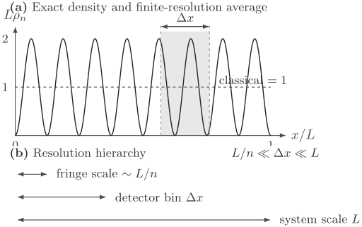
A high-$n$ density need not settle point by point. A detector bin satisfying $L/n\ll\Delta x\ll L$ resolves the classical spatial scale but not each quantum fringe, so its averaged probability approaches the uniform classical measure.

Weak convergence is not permission to discard all fine structure. An observable deliberately tuned to the wavelength-scale oscillations can retain an order-one quantum signal. The observable class must therefore be fixed before the limit is taken.

Wave Packets and Classical Trajectories

Stationary-state correspondence concerns distributions and frequencies. Particle-like motion requires a different state class, usually a packet localized in both position and momentum.

For

$$\hat H = \frac{\hat p^2}{2m} + V(\hat x),$$

Ehrenfest’s equations are exact:

$$\frac{d\langle\hat x\rangle}{dt} = \frac{\langle\hat p\rangle}{m}, \qquad \frac{d\langle\hat p\rangle}{dt} = -\langle V'(\hat x)\rangle.$$

They become a closed classical system only when

$$\langle V'(\hat x)\rangle \simeq V'(\langle\hat x\rangle).$$

Let

$$\bar x = \langle\hat x\rangle, \qquad \sigma_x^2 = \langle(\hat x-\bar x)^2\rangle.$$

Expanding the force about the packet center gives

$$\begin{aligned} \langle V'(\hat x)\rangle &= V'(\bar x) + \frac{1}{2} V'''(\bar x)\sigma_x^2 \\ &\quad + \frac{1}{6} V^{(4)}(\bar x) \langle(\hat x-\bar x)^3\rangle + \cdots. \end{aligned}$$

The packet center follows Newton’s equation while the higher-moment corrections remain small on the force scale of interest. The closure is exact for potentials at most quadratic, but generic packets spread, shear, or split in nonlinear potentials.

Three conclusions should be kept separate:

1. Center correspondence: $\bar x(t)$ and $\bar p(t)$ remain close to one classical trajectory.
2. Shape correspondence: the packet remains narrow and approximately Gaussian.
3. Observable correspondence: selected expectation values agree with a classical ensemble, even if one-packet localization has failed.

The first can fail while the third remains useful. A semiclassical propagator may accurately sum many classical trajectories after a single Gaussian packet has stretched beyond recognition. Ehrenfest Theorem Revisited derives the hierarchy of moments, while Wave Packets and Classical Trajectories owns the localization and spreading criteria. Coherent-State Semiclassics Preview compares one-packet variational propagation with trajectory-ensemble methods.

Fixed-Time and Long-Time Limits

A semiclassical approximation proved or derived for each fixed time need not remain accurate when time grows as $\epsilon$ decreases. Schematically, a statement such as

$$\lim_{\epsilon\to0} \sup_{0\le t\le T} \lvert Q_\epsilon(t)-Q_{\mathrm{cl}}(t) \rvert = 0$$

for every fixed $T$ does not establish the same result for $T=T(\epsilon)\to\infty$.

This order-of-limits issue is central:

$$\lim_{\epsilon\to0} \lim_{t\to\infty} Q_\epsilon(t) \qquad \text{and} \qquad \lim_{t\to\infty} \lim_{\epsilon\to0} Q_\epsilon(t)$$

need not agree. At long times, small frequency errors accumulate into phase errors; neighboring classical trajectories shear apart; caustics proliferate; discrete quantum recurrences can become visible; and exponentially small terms may become comparable to the nominal leading approximation.

For regular motion, packet deformation is often controlled by algebraic shear and by derivatives of the frequencies with respect to action. For chaotic motion, a linearized separation grows locally as

$$\delta z(t) \sim \delta z_0 e^{\lambda t},$$

where $\lambda$ is a positive Lyapunov exponent in the relevant region. If $L_z$ is a classical phase-space scale at which localization is lost, the estimate

$$t_{\mathrm E} \sim \frac{1}{\lambda} \log\left( \frac{L_z}{\delta z_0} \right)$$

defines an Ehrenfest time. For a minimum-uncertainty packet, $\delta z_0$ scales with a power of $\hbar$, so $t_{\mathrm E}$ grows only logarithmically with the inverse semiclassical parameter. The coefficient depends on which width, observable, flow direction, and phase-space norm define breakdown; there is no universal context-free prefactor.

The conclusion is not that “quantum trajectories become chaotic.” Closed quantum evolution is linear and does not possess classical trajectory separation in Hilbert space in that naive sense. Quantum signatures of classical chaos instead appear through spectral statistics, eigenfunction structure, periodic-orbit contributions, transport, scrambling diagnostics, and the time dependence of selected observables. Quantum Chaos Preview is the canonical introduction to those diagnostics.

Closed-System Semiclassics and Decoherence

Semiclassical approximation and decoherence solve different problems.

• Semiclassical approximation organizes closed-system amplitudes in powers or asymptotic scales of $\hbar/S_0$, often around classical trajectories or invariant manifolds.
• Coarse graining restricts which oscillations or phase-space structures an observable resolves.
• Decoherence suppresses locally observable interference between alternatives by entangling them with unobserved environmental degrees of freedom.

A closed high-action system can remain in a coherent superposition whose interference is visible to a sufficiently fine measurement. Conversely, environmental decoherence can make records robust even when a simple WKB expansion is not the right computational tool. In realistic classical behavior the mechanisms may cooperate, but neither should be smuggled into the assumptions of the other. See Decoherence and the Classical-Limit Bridge for the open-system analysis.

Method Crosswalk

The classical object and the appropriate notion of agreement depend on the quantum question.

Quantum question	Classical object	Appropriate comparison	Main method or repair
Bound-state energies	Actions and invariant tori	Level spacings, counting functions, smoothed spectral density	Bohr–Sommerfeld Quantization, EBK Quantization
Highly excited eigenstate density	Time-spent or invariant measure	Weak or coarse-grained convergence	WKB Approximation plus turning-point repair
Localized packet motion	Trajectory and stability matrix	Moments or smooth observables over a stated time	Ehrenfest analysis, Gaussian methods, coherent-state semiclassics
Propagator or transition amplitude	Boundary-value trajectories	Oscillatory asymptotics including phase and prefactor	Stationary Phase, Semiclassical Propagator
Tunneling probability	Complex or forbidden classical action	Logarithmic asymptotics of exponentially small terms	Forbidden-region WKB and connection formulas
Chaotic spectrum or transport	Unstable periodic orbits and classical correlations	Smoothed, statistical, or finite-time quantities	Periodic-orbit and quantum-chaos methods

The table also shows why “the quantum answer approaches the classical answer” is too coarse. A wavefunction is not a classical trajectory, an amplitude is not a probability density, and a discrete spectrum is not an orbit. Correspondence relates selected structures after the relevant representation and resolution have been specified.

How to Report a Semiclassical Result

For a calculation, simulation, or paper, a concise reliability statement can follow this order:

1. Nondimensionalize. Name the small parameter, such as $\epsilon=\hbar/(p_0L)$.
2. Define the family. State what changes and what remains fixed as $\epsilon\to0$.
3. Name the state class. Distinguish eigenstates, localized packets, mixtures, and trajectory-generated states.
4. Name the observables and resolution. State whether the claim is pointwise, weak, energy-smoothed, or detector-averaged.
5. State the time regime. Give fixed-time, one-period, Ehrenfest-time, or other scaling assumptions.
6. Give the leading classical object. Identify the orbit, torus, invariant measure, Liouville density, or trajectory sum.
7. Quantify the remainder. Report an asymptotic order, numerical residual, phase error, or empirical convergence test.
8. List singular sets. Note turning points, caustics, separatrices, resonances, bifurcations, and boundaries where the approximation changes form.

A numerical comparison should vary the dimensionless parameter while keeping the scaled classical problem fixed. Merely refining the numerical grid tests discretization error, not the semiclassical limit. Likewise, agreement of a probability with classical mechanics does not validate a phase-sensitive amplitude.

Common Misconceptions

“Taking ℏ to zero means setting it equal to zero”

The limit is singular. Setting $\hbar=0$ before constructing the asymptotics removes the derivative term or destroys the oscillatory phase whose stationary points generate classical mechanics.

“Large quantum number makes a state a classical trajectory”

A high-$n$ energy eigenstate is stationary up to phase and is generally spread over the classically allowed region. A localized trajectory requires a suitable superposition and a finite-time localization analysis.

“Rapid oscillations are physically absent”

They vanish only for an observable class that does not resolve them. A wavelength-sensitive probe can recover interference that a coarse detector averages away.

“Ehrenfest’s theorem proves classical motion”

The theorem gives exact equations for first moments, but those equations do not close for a nonlinear force unless higher moments remain negligible.

“Relative level spacing going to zero means absolute spacing goes to zero”

The harmonic oscillator has constant absolute spacing at fixed $\hbar$, and the box spacing grows with $n$. Classical spectral appearance depends on the comparison scale and measurement resolution.

“A good leading trajectory is enough”

Semiclassical amplitudes require stability prefactors, Maslov phases, branch sums, and uniformization near caustics. A small trajectory error can produce an order-one phase error when divided by $\hbar$.

“Classical chaos invalidates all semiclassics immediately”

Single-packet localization can fail rapidly, but trace formulas, trajectory sums, and statistical correspondence can remain informative in their own regimes.

“Decoherence and the semiclassical limit are the same”

Decoherence is an open-system suppression of accessible interference. Semiclassical asymptotics can be formulated for an exactly isolated, fully coherent system.

For a broader conceptual audit, see Common Misstatements About the Classical Limit.

Exercises

1. Nondimensionalize the Schrödinger equation

Starting from

$$\left[ -\frac{\hbar^2}{2m}\frac{d^2}{dx^2} + V_0 f(x/L) \right]\psi = E\psi,$$

choose $E_0$, define $p_0=\sqrt{mE_0}$, and obtain a dimensionless equation. Identify all remaining dimensionless parameters.

Solution

Set

$$\begin{aligned} y &= \frac{x}{L}, \\ \mathcal E &= \frac{E}{E_0}, \\ u &= \frac{V_0}{E_0}, \\ \epsilon &= \frac{\hbar}{p_0L}. \end{aligned}$$

Because

$$\frac{d^2}{dx^2} = \frac{1}{L^2} \frac{d^2}{dy^2}$$

and $p_0^2=mE_0$, division by $E_0$ gives

$$\left[ -\frac{\epsilon^2}{2} \frac{d^2}{dy^2} + u f(y) \right]\psi(y) = \mathcal E\psi(y).$$

The dimensionless data are $\epsilon$, the potential ratio $u$, the scaled energy $\mathcal E$, and any dimensionless shape parameters hidden in $f$. A clean semiclassical family sends $\epsilon\to0$ while the scaled potential and energy are held fixed.

2. Recover the classical frequency from EBK levels

Suppose a one-dimensional integrable system has $E=H(J)$ and

$$J_n = \hbar \left( n+\frac{\mu}{4} \right).$$

For fixed integer $r$, show that

$$\frac{E_{n+r}-E_n}{\hbar} = r\omega(J_n) + O(\hbar),$$

where $\omega=dH/dJ$. State the required joint limit.

Solution

The action spacing is

$$J_{n+r}-J_n = r\hbar.$$

Taylor expansion gives

$$\begin{aligned} H(J_n+r\hbar) &= H(J_n) + r\hbar H'(J_n) \\ &\quad + \frac{r^2\hbar^2}{2} H''(J_n) + O(\hbar^3). \end{aligned}$$

Therefore

$$\begin{aligned} \frac{E_{n+r}-E_n}{\hbar} &= rH'(J_n) + O(\hbar) \\ &= r\omega(J_n) + O(\hbar). \end{aligned}$$

The classical orbit is held fixed by taking $\hbar\to0$ and $n\to\infty$ with $J_n\to J$ and fixed $r$. Taking only $n\to\infty$ at fixed $\hbar$ generally changes the classical action.

3. Derive the classical time-spent density

In the allowed region of a one-dimensional bound orbit, take

$$\psi(x) \simeq \frac{C}{\sqrt{p(x)}} \cos\left( \frac{S(x)}{\hbar} -\frac{\pi}{4} \right).$$

Average over several oscillations, normalize over one allowed interval, and show that the result is $2/[T v(x)]$.

Solution

Oscillation averaging gives

$$\overline{\lvert\psi(x)\rvert^2} = \frac{C^2}{2p(x)}.$$

For a full classical period $T$, the travel time from the left turning point to the right one is $T/2$. Since $p=mv$,

$$\int_{x_-}^{x_+} \frac{dx}{p(x)} = \frac{1}{m} \int_{x_-}^{x_+} \frac{dx}{v(x)} = \frac{T}{2m}.$$

Normalization therefore requires

$$1 = \frac{C^2}{2} \frac{T}{2m}, \qquad C^2 = \frac{4m}{T}.$$

Substitution yields

$$\overline{\lvert\psi(x)\rvert^2} = \frac{2m}{Tp(x)} = \frac{2}{Tv(x)}.$$

Classically, the particle passes each interior interval $dx$ twice per period, so the fraction of a period spent there is $2\,dx/[Tv(x)]$. The formulas agree away from turning-point layers.

4. Estimate the first nonclassical force correction

Let a packet have mean $\bar x$, variance $\sigma_x^2$, and vanishing third central moment. Expand $\langle V'(\hat x)\rangle$ through second order in the packet displacement. Apply the result to

$$V(x) = \frac{1}{2}m\omega^2x^2 + \alpha x^4.$$

Solution

Write $\hat x=\bar x+\delta\hat x$, with $\langle\delta\hat x\rangle=0$. Taylor expansion gives

$$\langle V'(\hat x)\rangle = V'(\bar x) + \frac{1}{2} V'''(\bar x)\sigma_x^2 + \cdots.$$

For the quartic oscillator,

$$\begin{aligned} V'(x) &= m\omega^2x + 4\alpha x^3, \\ V'''(x) &= 24\alpha x. \end{aligned}$$

Hence

$$\langle V'(\hat x)\rangle \simeq m\omega^2\bar x + 4\alpha\bar x^3 + 12\alpha\bar x\sigma_x^2.$$

The last term is the leading width correction. It vanishes for a purely quadratic potential and grows as the packet spreads. Near $\bar x=0$ this particular correction vanishes by symmetry, so one should compare the first nonzero moment correction rather than divide mechanically by the classical force.

5. Estimate an Ehrenfest time

Assume a localized phase-space width grows as

$$\delta z(t) = \delta z_0e^{\lambda t}.$$

Find the time at which it reaches a classical scale $L_z$. If $\delta z_0/L_z=C\epsilon^{1/2}$, express the answer in terms of $\epsilon$ and explain why the coefficient is not universal.

Solution

Set $\delta z(t_{\mathrm E})=L_z$:

$$L_z = \delta z_0e^{\lambda t_{\mathrm E}}.$$

Thus

$$t_{\mathrm E} = \frac{1}{\lambda} \log\left( \frac{L_z}{\delta z_0} \right).$$

With $\delta z_0/L_z=C\epsilon^{1/2}$,

$$t_{\mathrm E} = \frac{1}{2\lambda} \log\left( \frac{1}{\epsilon} \right) -\frac{1}{\lambda}\log C.$$

The logarithmic scaling is robust under these assumptions, but the prefactor and additive term depend on the initial state’s width, the expanding direction, the chosen norm, the breakdown threshold, and the observable being monitored.

6. Distinguish pointwise and weak convergence in a box

For

$$\rho_n(x) = \frac{1}{L} \left[ 1-\cos\left( \frac{2n\pi x}{L} \right) \right],$$

show that no pointwise limit exists for generic fixed $x$, but that for every continuously differentiable $g$,

$$\int_0^L g(x)\rho_n(x)\,dx \longrightarrow \frac{1}{L} \int_0^L g(x)\,dx.$$

Obtain an explicit $O(1/n)$ bound on the oscillatory term.

Solution

At generic fixed $x$, the phase $2n\pi x/L$ continues to wind as $n$ increases, so the cosine does not settle to a single value. Thus $\rho_n(x)$ does not converge pointwise in general.

Let

$$k_n = \frac{2n\pi}{L}.$$

Let

$$I_n = \int_0^L g(x)\cos(k_nx)\,dx.$$

Integration by parts gives

$$\begin{aligned} I_n &= \left[ \frac{g(x)\sin(k_nx)}{k_n} \right]_0^L \\ &\quad -\frac{1}{k_n} \int_0^L g'(x)\sin(k_nx)\,dx. \end{aligned}$$

Because $\sin(k_nL)=\sin(2n\pi)=0$, the boundary term vanishes. Therefore

$$\begin{aligned} \lvert I_n\rvert &\le \frac{1}{k_n} \int_0^L\lvert g'(x)\rvert\,dx \\ &= O\left( \frac{1}{n} \right). \end{aligned}$$

The oscillatory contribution to the measured probability vanishes, leaving

$$\lim_{n\to\infty} \int_0^L g(x)\rho_n(x)\,dx = \frac{1}{L} \int_0^L g(x)\,dx.$$

This proves weak convergence for the stated observable class without claiming pointwise convergence.

References

1. M. V. Berry and K. E. Mount, “Semiclassical approximations in wave mechanics”, Reports on Progress in Physics 35, 315–397 (1972). Broad review of WKB, classical correspondence, turning points, and multidimensional semiclassics.
2. M. V. Berry, “Semi-Classical Mechanics in Phase Space: A Study of Wigner’s Function”, Philosophical Transactions of the Royal Society A 287, 237–271 (1977). Semiclassical phase-space measures, eigenstates, and classical invariant sets.
3. R. G. Littlejohn, “The semiclassical evolution of wave packets”, Physics Reports 138, 193–291 (1986). Systematic treatment of localized states, classical transport, and long-time limitations.
4. M. S. Child, Semiclassical Mechanics with Molecular Applications, 2nd ed. (Oxford University Press, 2014). Action quantization, correspondence of frequencies and matrix elements, and molecular applications.
5. M. Brack and R. K. Bhaduri, Semiclassical Physics, 2nd ed. (Westview Press, 2003). Spectral densities, periodic orbits, and regular and chaotic semiclassical systems.
6. M. C. Gutzwiller, Chaos in Classical and Quantum Mechanics (Springer, 1990). Classical instability, semiclassical propagation, periodic orbits, and quantum chaos.
7. G. P. Berman and G. M. Zaslavsky, “Condition of stochasticity in quantum nonlinear systems”, Physica A 91, 450–460 (1978). Early analysis of logarithmic correspondence times in unstable dynamics.
8. W. H. Zurek, “Decoherence, einselection, and the quantum origins of the classical”, Reviews of Modern Physics 75, 715–775 (2003). Authoritative review separating environmental decoherence from closed-system classical limits.
9. L. D. Landau and E. M. Lifshitz, Quantum Mechanics: Non-Relativistic Theory, 3rd ed. (Butterworth-Heinemann, 1981). Standard WKB correspondence between highly excited bound states and classical motion.
10. V. I. Arnold, Mathematical Methods of Classical Mechanics, 2nd ed. (Springer, 1989). Action-angle variables, invariant tori, and the classical structures used in EBK correspondence.