WKB in Classically Allowed Regions

In a classically allowed region, the energy lies above the potential and the local classical momentum is real. Leading WKB then represents the wavefunction as a coherent sum of right- and left-moving oscillatory branches. Each branch carries constant probability current, while its density grows where the corresponding classical motion slows.

This page is the operational home for those allowed-region branches: how to orient them, normalize their flux, combine them into standing waves, interpret the factor $p^{-1/2}$, and decide where the local formula is trustworthy. WKB in Classically Forbidden Regions is the exponential companion. WKB Approximation owns the order-by-order derivation, Turning Points and Connection Formulas owns the Airy repair where $p\to0$, and Bohr–Sommerfeld Quantization owns the global bound-state condition obtained after two such repairs.

The Local Oscillatory Basis

Consider the stationary one-dimensional Schrödinger equation

$$\left[ - \frac{\hbar^2}{2m} \frac{d^2}{dx^2} + V(x) \right]\psi(x) = E\psi(x),$$

with real $V(x)$. On an open interval $I$ where

$$E-V(x)\gt0,$$

define the positive local momentum and wavenumber

$$\begin{aligned} p(x) &= \sqrt{2m\bigl(E-V(x)\bigr)}, \\ k(x) &= \frac{p(x)}{\hbar}. \end{aligned}$$

Choose an arbitrary reference point $x_*\in I$ and define the accumulated phase

$$\theta(x;x_*) = \frac{1}{\hbar} \int_{x_*}^{x} p(s)\,ds.$$

The leading allowed-region WKB basis is

$$u_\pm(x) = \frac{1}{\sqrt{p(x)}} \exp\left[ \pm i\theta(x;x_*) \right].$$

Thus the general local solution is

$$\begin{aligned} \psi_{\mathrm{WKB}}(x) \approx{}& C_+u_+(x) \\ &+ C_-u_-(x). \end{aligned}$$

The $+$ branch has phase gradient $+p$ and the $-$ branch has phase gradient $-p$. For the Hamiltonian $H=p^2/(2m)+V$, their ray velocities are therefore

$$v_\pm(x) = \pm\frac{p(x)}{m}.$$

This direction assignment follows from current, not from visual inspection of a real-valued snapshot. The local action–phase dictionary is developed in Classical Action and Quantum Phase.

The reference point is a convention

Changing $x_*$ changes $\theta$ by a constant. If

$$\theta(x;\widetilde x_*) = \theta(x;x_*)-\alpha,$$

then the same wavefunction is obtained by

$$\widetilde C_+ = C_+e^{i\alpha}, \qquad \widetilde C_- = C_-e^{-i\alpha}.$$

Only relative phases fixed by boundary data or matching are observable. A lower limit written without explanation is not a physical origin of action.

Probability Current and Branch Direction

For a real scalar potential, the one-dimensional current is

$$j = \frac{\hbar}{m} \operatorname{Im} \left( \psi^*\frac{d\psi}{dx} \right).$$

Its general derivation and continuity equation belong to Probability Current. Applied to the WKB basis,

$$\frac{u_\pm'}{u_\pm} = - \frac{p'}{2p} \pm i\frac{p}{\hbar}.$$

Since $\lvert u_\pm\rvert^2=1/p$, each basis function carries

$$j[u_\pm] = \pm\frac{1}{m}.$$

For the two-branch superposition with constant coefficients,

$$j_{\mathrm{WKB}} = \frac{ \lvert C_+\rvert^2 - \lvert C_-\rvert^2 }{m}.$$

The interference terms cancel from the current. They do not cancel from the density.

Flux-normalized branches

It is often convenient in scattering calculations to absorb $\sqrt m$ into the basis:

$$\chi_\pm(x) = \sqrt{\frac{m}{p(x)}} \exp\left[ \pm i\theta(x;x_*) \right].$$

Then

$$j[\chi_\pm] = \pm1.$$

These are unit-flux rather than unit-norm states. Stationary scattering states are generally not square-integrable, so flux normalization is the useful convention. Whenever amplitudes from different asymptotic regions are compared, current ratios, not coefficient magnitudes alone, determine reflection and transmission probabilities.

Traveling waves and standing waves

The density of the general WKB combination is

$$\begin{aligned} \lvert\psi_{\mathrm{WKB}}\rvert^2 ={}& \frac{1}{p} \left( \lvert C_+\rvert^2 + \lvert C_-\rvert^2 \right) \\ &+ \frac{2}{p} \operatorname{Re} \left[ C_+C_-^* e^{2i\theta} \right]. \end{aligned}$$

A pure branch has nonzero current and a smooth density envelope. If $\lvert C_+\rvert=\lvert C_-\rvert$, the net current vanishes and the wavefunction can be written, up to a constant overall phase, as

$$\psi_{\mathrm{stand}}(x) = \frac{B}{\sqrt{p(x)}} \cos\bigl(\theta(x)+\delta\bigr).$$

This is a standing wave built from two opposite fluxes. Zero net current does not mean that the semiclassical momentum is zero; it means that equal counterpropagating currents cancel.

Why the Amplitude Scales as Inverse Square Root of Momentum

For one traveling branch, write

$$\psi(x) = A(x)e^{\pm i\theta(x)}.$$

Its leading current is

$$j \approx \pm \frac{p}{m} \lvert A\rvert^2.$$

Stationarity requires $dj/dx=0$, so

$$\frac{d}{dx} \left( p\lvert A\rvert^2 \right) = 0.$$

Therefore

$$\lvert A(x)\rvert \propto \frac{1}{\sqrt{p(x)}}.$$

This current argument gives the same transport factor as the systematic expansion on the canonical WKB page. It also supplies the physical interpretation:

$$\begin{aligned} \rho_\pm(x) &= \frac{\lvert C_\pm\rvert^2}{p(x)}, \\ j_\pm &= \rho_\pm v_\pm = \pm\frac{\lvert C_\pm\rvert^2}{m}. \end{aligned}$$

Where $p$ is smaller, the ray velocity is smaller and a fixed flux requires a larger probability density.

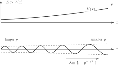
Across a smooth allowed region, decreasing $p(x)$ increases both the local de Broglie wavelength and the envelope $p(x)^{-1/2}$. The amplitude growth preserves current; it is not an independent probability source.

Classical dwell-time density

The same inverse-velocity weighting appears in classical mechanics. For periodic motion between two turning points, a classical trajectory crosses an interior point twice per period $T$. Its normalized dwell-time density is

$$P_{\mathrm{cl}}(x) = \frac{2}{T\lvert v(x)\rvert} = \frac{2m}{T p(x)}.$$

For a standing WKB wave,

$$\lvert\psi_{\mathrm{stand}}\rvert^2 = \frac{\lvert B\rvert^2}{p} \cos^2(\theta+\delta).$$

Coarse-graining over several local oscillations uses

$$\overline{\cos^2(\theta+\delta)} = \frac12,$$

and therefore

$$\overline{\lvert\psi_{\mathrm{stand}}\rvert^2} = \frac{\lvert B\rvert^2}{2p(x)}.$$

After normalization, this agrees with the classical dwell-time density in the semiclassical regime. The agreement concerns a locally averaged density. The exact quantum density retains nodes and interference fringes.

Validity Inside an Allowed Region

The condition $E\gt V$ makes the WKB solution oscillatory, but it does not by itself make WKB accurate. The local momentum must also vary slowly on the scale of a wavelength.

The common first-derivative test

The standard dimensionless parameter is

$$\epsilon_1(x) = \left\lvert \hbar\frac{p'(x)}{p^2(x)} \right\rvert \ll1.$$

Since

$$p' = - \frac{mV'}{p},$$

this can be written

$$\epsilon_1 = \frac{ \hbar m\lvert V'\rvert }{ p^3 }.$$

Equivalently, the fractional change in $p$ across a reduced wavelength $\hbar/p$ must be small. Numerical factors of $2\pi$ differ depending on whether one speaks of the reduced wavelength or the full de Broglie wavelength; the asymptotic requirement is the same.

A residual test that sees curvature

The stationary equation can be written

$$\psi'' + \frac{p^2}{\hbar^2}\psi = 0.$$

Substituting either leading branch $u_\pm$ gives

$$\begin{aligned} u_\pm'' + \frac{p^2}{\hbar^2}u_\pm ={}& \biggl[ \frac34 \left( \frac{p'}{p} \right)^2 \\ &- \frac12 \frac{p''}{p} \biggr]u_\pm. \end{aligned}$$

A direct dimensionless residual is therefore

$$\mathcal R(x) = \frac{\hbar^2}{p^2} \left[ \frac34 \left( \frac{p'}{p} \right)^2 - \frac12 \frac{p''}{p} \right].$$

Leading WKB requires $\lvert\mathcal R\rvert\ll1$ on the region of interest. This exposes a limitation of checking only $\epsilon_1$: at a point where $p'=0$, the first-derivative test vanishes even though $p''$ may still generate an error.

One can track the two derivative scales separately:

$$\epsilon_1 = \frac{\hbar\lvert p'\rvert}{p^2}, \qquad \epsilon_2 = \frac{\hbar^2\lvert p''\rvert}{p^3}.$$

For a generic smooth profile with one variation length, $\epsilon_2$ is of the same asymptotic order as $\epsilon_1^2$. Near special points or on multiscale profiles, it need not be.

Local accuracy is not global phase accuracy

Even when the residual is small everywhere, a small local correction to the wavenumber can accumulate over many oscillations. A phase-sensitive calculation should therefore report both:

1. a local slow-variation or residual estimate;
2. an estimate of the integrated phase error over the interval used.

For a spectrum, resonance, or interferometer, an order-one phase error can matter even when the relative error in a large action is small. The general distinction between local control and accumulated observable error is developed in Small Parameters and Error Estimates.

Distance from turning points

At a simple turning point $x_t$,

$$p(x_t)=0,$$

so the amplitude and derivative tests fail. The leading allowed-region formula is valid only on subintervals that stay outside the local turning-point layer. Extending $p^{-1/2}$ to $x_t$ and interpreting its divergence physically is incorrect; the exact wavefunction remains finite in the usual simple-turning-point problem.

Worked Examples

Constant potential

Let $V(x)=V_0$ and $E\gt V_0$. Then

$$p_0 = \sqrt{2m(E-V_0)}$$

is constant, so

$$\theta(x;x_*) = \frac{p_0(x-x_*)}{\hbar}.$$

The WKB branches are plane waves,

$$u_\pm(x) = \frac{1}{\sqrt{p_0}} e^{\pm ip_0(x-x_*)/\hbar},$$

and they solve the Schrödinger equation exactly. Here $p'=p''=0$, so the residual vanishes. This benchmark checks branch signs, current normalization, and phase conventions.

Linear ramp away from its turning point

Take

$$V(x) = V_0+Fx, \qquad F\gt0,$$

and define

$$x_t = \frac{E-V_0}{F}.$$

The region $x\lt x_t$ is allowed. Its momentum is

$$p(x) = \sqrt{2mF(x_t-x)}.$$

Using the turning point only as a phase reference,

$$\begin{aligned} \zeta(x) &= \frac{1}{\hbar} \int_x^{x_t} p(s)\,ds \\ &= \frac{ 2\sqrt{2mF} }{ 3\hbar } (x_t-x)^{3/2}. \end{aligned}$$

Away from $x_t$, the oscillatory basis is

$$u_\pm(x) = \frac{ e^{\mp i\zeta(x)} }{ \bigl[2mF(x_t-x)\bigr]^{1/4} }.$$

The first-derivative parameter is

$$\epsilon_1(x) = \frac{\hbar}{ 2\sqrt{2mF} (x_t-x)^{3/2} }.$$

Introduce the Airy length

$$\ell_F = \left( \frac{\hbar^2}{2mF} \right)^{1/3}.$$

Then

$$\epsilon_1 = \frac12 \left( \frac{\ell_F}{x_t-x} \right)^{3/2}.$$

The allowed-region WKB formula is controlled for $x_t-x\gg\ell_F$. Inside a layer of order $\ell_F$, the exact Airy solution, not the isolated WKB branches, supplies the uniform description.

Harmonic oscillator interior

For

$$V(x) = \frac12m\omega^2x^2,$$

write the energy as

$$E = \frac12m\omega^2a^2.$$

The allowed interval is $\lvert x\rvert\lt a$, with

$$p(x) = m\omega\sqrt{a^2-x^2}.$$

Taking the origin as phase reference gives

$$\begin{aligned} \int_0^x p(s)\,ds ={}& \frac{m\omega}{2} \bigg[ x\sqrt{a^2-x^2} \\ &+ a^2\arcsin\left(\frac{x}{a}\right) \bigg]. \end{aligned}$$

The amplitude envelope is

$$\frac{1}{\sqrt{p(x)}} = \frac{1}{ \sqrt{m\omega} \left(a^2-x^2\right)^{1/4} }.$$

It grows toward $\pm a$, warning that the interior approximation is approaching its turning-point failure. The first-derivative parameter is

$$\epsilon_1(x) = \frac{ \hbar\lvert x\rvert }{ m\omega \left(a^2-x^2\right)^{3/2} }.$$

At $x=0$, this parameter vanishes by symmetry, but WKB is not thereby exact. The curvature term in $\mathcal R$ remains, and the relevant interior action scale is

$$p(0)a = m\omega a^2 = \frac{2E}{\omega}.$$

The interior becomes semiclassical when $E/(\hbar\omega)$ is large. After oscillation averaging and normalization, the WKB standing-wave density tends to

$$\overline{\lvert\psi(x)\rvert^2} \approx \frac{1}{ \pi\sqrt{a^2-x^2} },$$

which is exactly the normalized classical dwell-time density away from the turning-point layers. The exact model is developed in Quantum Harmonic Oscillator; its global WKB spectrum and turning-point phases are standard applications of Bohr–Sommerfeld Quantization.

High-energy phase through a smooth weak potential

Suppose $\lvert V(x)\rvert/E$ is small throughout an allowed interval and define

$$p_0 = \sqrt{2mE}.$$

Expanding the local momentum gives

$$\begin{aligned} p(x) &= p_0 \sqrt{1-\frac{V(x)}{E}} \\ &\approx p_0 - \frac{m}{p_0}V(x). \end{aligned}$$

The accumulated phase is therefore

$$\theta(x;x_*) \approx \frac{p_0(x-x_*)}{\hbar} - \frac{m}{\hbar p_0} \int_{x_*}^{x} V(s)\,ds.$$

The first term is free propagation; the second is the leading phase delay or advance. The amplitude changes more mildly:

$$\frac{1}{\sqrt{p(x)}} \approx \frac{1}{\sqrt{p_0}} \left[ 1+ \frac{V(x)}{4E} \right].$$

This local single-branch approximation does not by itself compute the reflected amplitude. Reflection is branch conversion determined by global variation, boundaries, or complex turning-point structure.

Practical Workflow

For an allowed-region WKB calculation:

1. Identify each connected interval on which $E-V(x)\gt0$.
2. Choose the positive magnitude $p(x)=\sqrt{2m(E-V)}$.
3. Select a convenient phase reference and record its convention.
4. Construct both $p^{-1/2}e^{\pm i\theta}$ branches before imposing boundary data.
5. Use current to label directions and normalize scattering branches.
6. Evaluate both the common slow-variation parameter and, when needed, the direct residual.
7. Exclude turning-point layers and abrupt interfaces from the local formula.
8. Determine $C_+$ and $C_-$ from physical boundaries, matching, or incoming-wave conditions.
9. Track accumulated phase accuracy when the observable is phase-sensitive.
10. Compare with an exact limit, conservation law, numerical solution, or higher-order approximation.

Common Mistakes

• Calling a region semiclassical merely because $E\gt V(x)$.
• Dropping the factor $p^{-1/2}$ and thereby violating constant current.
• Assigning direction from the sign of $x$ rather than the sign of the phase gradient or current.
• Treating $C_+$ and $C_-$ as probabilities before converting them to fluxes.
• Assuming zero current for a standing wave means zero local momentum.
• Interpreting the oscillatory density as the classical probability density without coarse-graining.
• Treating the arbitrary lower limit in the action integral as physical.
• Checking only $p'$ at a symmetry point and ignoring curvature.
• Extending the allowed-region formula into a turning point.
• Applying smooth WKB across a discontinuous potential step.
• Assuming a small local residual guarantees a negligible accumulated phase error.
• Expecting a one-branch ansatz to determine an exponentially small reflected branch.

Exercises

1. Current carried by each branch

For

$$u_\pm(x) = \frac{1}{\sqrt{p(x)}} \exp\left[ \pm \frac{i}{\hbar} \int^x p(s)\,ds \right],$$

show that $j[u_\pm]=\pm1/m$.

Solution

Differentiate:

$$u_\pm' = \left( - \frac{p'}{2p} \pm i\frac{p}{\hbar} \right)u_\pm.$$

The logarithmic-amplitude term is real, so only the phase-gradient term contributes to the imaginary part. Since $\lvert u_\pm\rvert^2=1/p$,

$$\begin{aligned} j[u_\pm] &= \frac{\hbar}{m} \operatorname{Im} \left( u_\pm^*u_\pm' \right) \\ &= \frac{\hbar}{m} \frac{1}{p} \left( \pm\frac{p}{\hbar} \right) \\ &= \pm\frac1m. \end{aligned}$$

2. Current and fringes in a two-branch state

For $\psi=C_+u_++C_-u_-$, derive the current and density. What happens when $\lvert C_+\rvert=\lvert C_-\rvert$?

Solution

Using $u_-=u_+^*$ for real $p$ gives

$$j = \frac{ \lvert C_+\rvert^2 - \lvert C_-\rvert^2 }{m}.$$

The cross terms cancel from $j$. The density is

$$\begin{aligned} \lvert\psi\rvert^2 ={}& \frac{ \lvert C_+\rvert^2 + \lvert C_-\rvert^2 }{p} \\ &+ \frac{2}{p} \operatorname{Re} \left[ C_+C_-^*e^{2i\theta} \right]. \end{aligned}$$

Equal branch magnitudes give $j=0$ but leave the interference term. The state is a standing wave composed of equal and opposite currents.

3. Invariance under a new phase reference

Let the phase be redefined by $\widetilde\theta=\theta-\alpha$. Find the transformed coefficients that leave $\psi$ unchanged.

Solution

Require

$$\begin{aligned} C_+e^{i\theta} + C_-e^{-i\theta} ={}& \widetilde C_+ e^{i(\theta-\alpha)} \\ & + \widetilde C_- e^{-i(\theta-\alpha)}. \end{aligned}$$

Matching the two independent branches gives

$$\widetilde C_+ = C_+e^{i\alpha}, \qquad \widetilde C_- = C_-e^{-i\alpha}.$$

The reference change is absorbed into constant coefficient phases, so currents and densities are unchanged.

4. Width of the linear turning-point layer

For $V(x)=V_0+Fx$ with $F\gt0$, show that

$$\begin{aligned} \epsilon_1 &= \frac12 \left( \frac{\ell_F}{x_t-x} \right)^{3/2}, \\ \ell_F &= \left( \frac{\hbar^2}{2mF} \right)^{1/3}. \end{aligned}$$

What distance from $x_t$ is required for leading WKB?

Solution

In the allowed region,

$$p = \sqrt{2mF(x_t-x)}.$$

Its derivative has magnitude

$$\lvert p'\rvert = \frac{\sqrt{2mF}}{ 2\sqrt{x_t-x} }.$$

Therefore

$$\begin{aligned} \epsilon_1 &= \hbar \frac{\lvert p'\rvert}{p^2} \\ &= \frac{\hbar}{ 2\sqrt{2mF} (x_t-x)^{3/2} } \\ &= \frac12 \left( \frac{\ell_F}{x_t-x} \right)^{3/2}. \end{aligned}$$

Leading WKB requires $x_t-x\gg\ell_F$. At distances of order $\ell_F$, an Airy approximation is required.

5. Harmonic-oscillator dwell-time density

A classical oscillator of amplitude $a$ has speed

$$\lvert v(x)\rvert = \omega\sqrt{a^2-x^2}$$

and period $T=2\pi/\omega$. Derive its normalized position density and compare it with the coarse-grained WKB envelope.

Solution

The oscillator crosses each interior point twice per period, so

$$P_{\mathrm{cl}}(x) = \frac{2}{T\lvert v(x)\rvert}.$$

Substitution gives

$$P_{\mathrm{cl}}(x) = \frac{1}{ \pi\sqrt{a^2-x^2} }.$$

The normalization follows from

$$\int_{-a}^{a} \frac{dx}{ \pi\sqrt{a^2-x^2} } = 1.$$

Since $p=m\lvert v\rvert$, a standing WKB wave has coarse-grained density proportional to $1/p$, hence to $1/\sqrt{a^2-x^2}$. Normalization makes it equal to $P_{\mathrm{cl}}$ away from the turning-point layers.

6. Leading phase shift from a weak smooth potential

For $E\gt\lvert V(x)\rvert$ with $\lvert V\rvert/E\ll1$, expand $p(x)=\sqrt{2m(E-V)}$ through first order in $V/E$ and obtain the phase relative to free propagation.

Solution

With $p_0=\sqrt{2mE}$,

$$\begin{aligned} p(x) &= p_0 \left( 1-\frac{V}{E} \right)^{1/2} \\ &\approx p_0 \left( 1-\frac{V}{2E} \right) \\ &= p_0-\frac{m}{p_0}V(x). \end{aligned}$$

Integrating and dividing by $\hbar$ gives

$$\begin{aligned} \theta(x;x_*) \approx{}& \frac{p_0(x-x_*)}{\hbar} \\ & - \frac{m}{\hbar p_0} \int_{x_*}^{x} V(s)\,ds. \end{aligned}$$

The second term is the leading phase relative to a free wave. Its sign follows the sign of $V$: a positive potential lowers the local momentum and reduces the accumulated phase.

References

1. L. D. Landau and E. M. Lifshitz, Quantum Mechanics: Non-Relativistic Theory, 3rd ed. (Butterworth-Heinemann, 1981). WKB waves, current interpretation, turning points, and quantization.
2. C. M. Bender and S. A. Orszag, Advanced Mathematical Methods for Scientists and Engineers I (Springer, 1999). Liouville–Green asymptotics, error structure, and connection methods.
3. M. V. Berry and K. E. Mount, “Semiclassical approximations in wave mechanics”, Reports on Progress in Physics 35, 315–397 (1972). Phase-integral interpretation, branch structure, and semiclassical validity.
4. F. W. J. Olver, Asymptotics and Special Functions (A K Peters, 1997). Error-controlled Liouville–Green approximations and uniform asymptotics.
5. J. Heading, An Introduction to Phase-Integral Methods (Methuen, 1962). Traveling-wave bases, phase integrals, and connection theory.
6. R. Shankar, Principles of Quantum Mechanics, 2nd ed. (Springer, 1994). WKB wavefunctions, bound-state interpretation, and standard examples.