Multidimensional WKB Preview

Multidimensional WKB replaces the single position coordinate of ordinary WKB by a family of classical rays in configuration space. The rapidly varying phase solves a Hamilton–Jacobi, or eikonal, equation. The slowly varying amplitude is transported by conservation of probability flux through a ray tube.

That concise statement hides the new difficulty. In one dimension, a local momentum sign usually labels the two branches. In several dimensions, neighboring rays can focus, intersect in configuration space, and generate several action branches at the same point. A single WKB amplitude then becomes singular at a caustic even though the exact wave remains finite.

This page is an advanced operational preview. It owns the stationary multidimensional ansatz, its transport law, and the ray/caustic interpretation. Hamilton–Jacobi Theory owns the classical action equation, EBK Quantization owns global quantization on invariant tori, and Van Vleck Determinant owns the endpoint stability prefactor for propagators.

Stationary WKB Ansatz

Consider a scalar particle in $d$ Euclidean dimensions:

$$\left[ - \frac{\hbar^2}{2m}\nabla^2 + V(\mathbf q) \right] \psi(\mathbf q) = E\psi(\mathbf q).$$

In a region with a rapidly varying phase and a slowly varying envelope, write one local branch as

$$\psi(\mathbf q) = A(\mathbf q) \exp\left[ \frac{i}{\hbar} S(\mathbf q) \right].$$

For the leading allowed-region construction, $S$ and $A$ may be taken real. The phase function $S$ has units of action.

Define the eikonal residual

$$\mathcal E[S] = \frac{ \lvert\nabla S\rvert^2 }{2m} + V-E$$

and the transport expression

$$\mathcal T[A,S] = 2\nabla A\cdot\nabla S + A\nabla^2S.$$

Direct substitution into the Schrödinger equation gives

$$\begin{aligned} 0 ={}& A\mathcal E[S] \\ &- \frac{i\hbar}{2m} \mathcal T[A,S] \\ &- \frac{\hbar^2}{2m} \nabla^2A. \end{aligned}$$

This equation is exact for the ansatz. The WKB approximation organizes its three terms by how many slow derivatives or explicit powers of $\hbar$ they contain.

Eikonal Equation

At leading order,

$$\mathcal E[S]=0,$$

or

$$\frac{ \lvert\nabla S\rvert^2 }{2m} + V(\mathbf q) = E.$$

Define the local branch momentum by

$$\mathbf p(\mathbf q) = \nabla S(\mathbf q).$$

Then

$$\lvert\mathbf p\rvert = \sqrt{ 2m \bigl(E-V(\mathbf q)\bigr) }.$$

This is the time-independent Hamilton–Jacobi equation. It determines the phase surfaces $S(\mathbf q)=\text{constant}$ and the momentum field normal to them.

The equation determines only the magnitude of $\nabla S$ directly. Boundary data select its direction and may generate several solutions. A point reached by several classical rays generally has several local action branches $S_\gamma$, not one globally single-valued phase.

Characteristics Are Classical Rays

The characteristics of the eikonal equation are classical trajectories at energy $E$. With

$$H(\mathbf q,\mathbf p) = \frac{\lvert\mathbf p\rvert^2}{2m} + V(\mathbf q),$$

they obey

$$\begin{aligned} \dot{\mathbf q} &= \frac{\partial H}{\partial\mathbf p} = \frac{\mathbf p}{m}, \\ \dot{\mathbf p} &= - \frac{\partial H}{\partial\mathbf q} = - \nabla V. \end{aligned}$$

Along a characteristic,

$$\mathbf p=\nabla S,$$

and the action changes according to

$$\frac{dS}{dt} = \mathbf p\cdot\dot{\mathbf q}.$$

Thus the eikonal partial differential equation can be solved locally by launching a family of classical rays from suitable boundary data and accumulating the action along them.

The phase surfaces are wavefronts. Rays point in the direction of $\nabla S$ and therefore cross the wavefronts orthogonally for the scalar Hamiltonian used here. In magnetic fields, anisotropic media, band Hamiltonians, or constrained coordinates, velocity need not be parallel to canonical momentum; the ray construction must then use the full Hamiltonian characteristics.

Transport Equation

At the next order, set

$$\mathcal T[A,S]=0.$$

The amplitude obeys

$$2\nabla S\cdot\nabla A + A\nabla^2S = 0.$$

Multiplying by $A$ gives the conservation form

$$\nabla\cdot \left( A^2\nabla S \right) = 0.$$

For a real leading amplitude, the probability current is

$$\mathbf j = \frac{\hbar}{m} \operatorname{Im} \left( \psi^*\nabla\psi \right) \approx \frac{A^2}{m} \nabla S.$$

Consequently,

$$\nabla\cdot\mathbf j \approx 0.$$

The amplitude is not a decorative normalization. It is the factor that makes the classical ray family carry conserved quantum probability flux.

Evolution along one ray

Let

$$\mathbf v = \frac{\nabla S}{m}.$$

The transport equation becomes

$$\mathbf v\cdot\nabla A + \frac{A}{2} \nabla\cdot\mathbf v = 0.$$

Since $d/dt=\mathbf v\cdot\nabla$ along a ray,

$$\frac{d\ln A}{dt} = - \frac12 \nabla\cdot\mathbf v.$$

An expanding ray family has $\nabla\cdot\mathbf v\gt0$ and a decreasing amplitude. A focusing family has $\nabla\cdot\mathbf v\lt0$ and an increasing amplitude.

Ray Tubes and Jacobians

Label rays by $\boldsymbol\alpha=(\alpha_1,\ldots,\alpha_{d-1})$ and use $t$ as a parameter along them:

$$\mathbf q = \mathbf q(t,\boldsymbol\alpha).$$

The configuration-space ray Jacobian is

$$J_{\mathbf q} = \left| \det \frac{ \partial\mathbf q }{ \partial(t,\boldsymbol\alpha) } \right|.$$

Before the projection becomes singular,

$$\frac{d\ln J_{\mathbf q}}{dt} = \nabla\cdot\mathbf v.$$

Combining this relation with amplitude transport gives

$$\frac{d}{dt} \left( A^2J_{\mathbf q} \right) = 0.$$

Hence

$$\begin{aligned} A(t,\boldsymbol\alpha) ={}& A(t_0,\boldsymbol\alpha) \\ &\times \left[ \frac{ J_{\mathbf q}(t_0,\boldsymbol\alpha) }{ J_{\mathbf q}(t,\boldsymbol\alpha) } \right]^{1/2}. \end{aligned}$$

Equivalently, for a thin ray tube crossing a transverse area element $d\Sigma$,

$$A^2v_\perp\,d\Sigma = \text{constant},$$

where $v_\perp$ is the velocity component through that cross section.

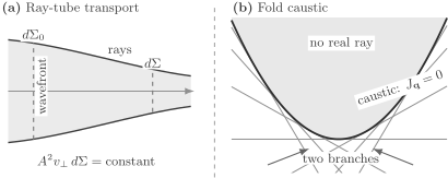
Left: transport conserves $A^2v_\perp d\Sigma$, so a narrowing ray tube increases the WKB amplitude. Right: at a fold caustic, the ray-label map has $J_{\mathbf q}=0$; two real branches merge and the isolated-branch amplitude diverges, while the exact wave is described by a uniform approximation.

The Jacobian here is a configuration-space projection Jacobian. Hamiltonian flow remains nonsingular and volume-preserving in full phase space. A caustic occurs because a smooth phase-space manifold projects singularly onto configuration space, not because classical phase-space evolution itself ceases to exist.

One-Dimensional Limit

In one dimension, a stationary branch carries

$$j \approx \frac{A^2p}{m}.$$

Constant flux therefore requires

$$A \propto \frac{1}{\sqrt{\lvert p\rvert}}.$$

The familiar WKB prefactor is thus the one-dimensional form of ray-tube transport. There is no transverse area, but the local speed still changes the amount of probability density needed to carry a fixed current.

Basic Examples

Plane wave

For $V=V_0$ and $E\gt V_0$, choose a constant momentum satisfying

$$\frac{\lvert\mathbf p_0\rvert^2}{2m} + V_0 = E.$$

Then

$$S(\mathbf q) = \mathbf p_0\cdot\mathbf q$$

has

$$\nabla^2S=0.$$

The transport equation permits constant $A$, and the WKB branch is an exact plane-wave solution.

Radial outgoing wave

For a free particle outside a point source, take

$$S(\mathbf q)=pr, \qquad r=\lvert\mathbf q\rvert.$$

Radial flux through a sphere in $d$ dimensions gives

$$A^2 \frac{p}{m} r^{d-1} = \text{constant}.$$

Thus

$$A(r) \propto r^{-(d-1)/2}.$$

In three dimensions,

$$\psi_{\mathrm{out}}(r) \propto \frac{1}{r} \exp\left( \frac{ipr}{\hbar} \right).$$

The inverse-distance amplitude is the geometric spreading of a ray bundle, not an extra assumption about spherical waves. More generally, $r^{-(d-1)/2}$ is the leading large-$pr/\hbar$ radial amplitude; subleading inverse-radius terms are retained by the exact Bessel or Hankel solution.

Several classical paths

An obstacle, lensing potential, curved boundary, or nontrivial classical motion can send several rays to the same point. Each ray carries its own action and transport amplitude. Define its total semiclassical phase by

$$\Phi_\gamma = \frac{S_\gamma}{\hbar} - \frac{\pi}{2}\mu_\gamma.$$

The local semiclassical field is then a coherent branch sum rather than a single eikonal:

$$\psi(\mathbf q) \approx \sum_\gamma A_\gamma(\mathbf q) e^{i\Phi_\gamma}.$$

The integer $\mu_\gamma$ records caustic and representation phase changes under a chosen Maslov-index convention.

For each unordered pair, define

$$\mathcal I_{\gamma\gamma'} = A_\gamma A_{\gamma'}^* e^{i(\Phi_\gamma-\Phi_{\gamma'})}.$$

The probability contains the pair-interference terms

$$\begin{aligned} \lvert\psi\rvert^2 \approx{}& \sum_\gamma \lvert A_\gamma\rvert^2 \\ &+ 2 \sum_{\gamma<\gamma'} \operatorname{Re} \mathcal I_{\gamma\gamma'}. \end{aligned}$$

Classical rays organize the branches, but the branches still interfere quantum mechanically.

Caustics

A local action branch defines a Lagrangian manifold in phase space,

$$\Lambda = \left\{ (\mathbf q,\mathbf p) : \mathbf p=\nabla S(\mathbf q) \right\}.$$

The projection

$$\pi_{\mathbf q}: \Lambda\longrightarrow \text{configuration space}$$

can fail to be locally one-to-one. At such a point,

$$J_{\mathbf q}=0,$$

and the transport formula predicts

$$A\propto J_{\mathbf q}^{-1/2}.$$

The divergence is not a physical blow-up of the exact wave. It says that one configuration-space phase branch is a bad local representation.

Near a generic fold caustic, two stationary branches coalesce and an Airy-type uniform approximation replaces their separate divergent terms. Cusp caustics require a different canonical integral, often of Pearcey type. The detailed classification belongs to uniform asymptotics and Maslov theory; the practical lesson is simpler:

do not evaluate an isolated-branch WKB formula at a point where its ray Jacobian vanishes.

Crossing a caustic also changes the phase associated with the square-root amplitude. Maslov Index owns that bookkeeping.

Relation to Ray Optics

For a scalar Helmholtz field,

$$\left[ \nabla^2 + k_0^2n^2(\mathbf q) \right] u(\mathbf q) = 0,$$

the geometrical-optics ansatz is

$$u = a e^{ik_0\mathcal L}.$$

At leading order,

$$\lvert\nabla\mathcal L\rvert^2 = n^2,$$

and the optical amplitude obeys

$$\nabla\cdot \left( a^2\nabla\mathcal L \right) = 0.$$

The quantum stationary equation can likewise be written

$$\left[ \nabla^2 + \frac{p^2(\mathbf q)}{\hbar^2} \right] \psi = 0,$$

where

$$p^2(\mathbf q) = 2m \bigl(E-V(\mathbf q)\bigr).$$

The correspondence is:

• optical length $k_0\mathcal L$ corresponds to quantum phase $S/\hbar$;
• optical rays correspond to classical trajectories;
• optical intensity transport corresponds to probability-current transport;
• optical focal caustics correspond to singular configuration-space projections of classical trajectory families.

The analogy is structural, not complete. Electromagnetic waves have polarization, interfaces impose vector boundary conditions, and quantum mechanics allows classically forbidden propagation, spin transport, gauge phases, and operator-valued internal structure.

Time-Dependent Extension

For

$$\psi(\mathbf q,t) = A(\mathbf q,t) \exp\left[ \frac{i}{\hbar} S(\mathbf q,t) \right],$$

the leading phase satisfies

$$\frac{\partial S}{\partial t} + \frac{ \lvert\nabla S\rvert^2 }{2m} + V(\mathbf q,t) = 0.$$

The leading amplitude satisfies

$$\frac{\partial A}{\partial t} + \frac{\nabla S}{m}\cdot\nabla A + \frac{A}{2m}\nabla^2S = 0.$$

Writing $\rho=A^2$ gives

$$\frac{\partial\rho}{\partial t} + \nabla\cdot \left( \rho \frac{\nabla S}{m} \right) = 0.$$

This is the time-dependent ray-density transport law. The Semiclassical Propagator and Van Vleck Determinant reorganize the same geometry in terms of trajectories joining fixed endpoints.

Forbidden Regions in Several Dimensions

In a forbidden region, a decaying branch may be written

$$\psi(\mathbf q) \sim B(\mathbf q) \exp\left[ - \frac{1}{\hbar} W(\mathbf q) \right].$$

The leading real decay action obeys

$$\lvert\nabla W\rvert^2 = 2m \bigl(V(\mathbf q)-E\bigr).$$

This is an imaginary-momentum eikonal equation. In more than one dimension, the exponent is not generally obtained by choosing an arbitrary straight path and integrating

$$\sqrt{2m(V-E)}.$$

Boundary data and the eikonal equation determine the relevant decay surface and dominant paths. Several complex or Euclidean trajectories can compete, and Stokes switching can change which branches contribute. Detailed multidimensional tunneling is therefore naturally connected to instanton and complex-trajectory methods rather than to a naive line integral.

From Local Rays to Global Quantization

The eikonal and transport equations are local. A global wavefunction must also satisfy:

• boundary and matching conditions;
• single-valuedness or bundle-valued consistency;
• phase changes at caustics;
• topology of the underlying classical invariant set;
• interference among all relevant branches.

For a classically integrable system, invariant tori and their cycles provide the global structure. EBK Quantization imposes phase consistency on those cycles and includes the Maslov correction.

For nonintegrable systems, one generally cannot introduce one global action function or one set of action-angle variables covering the motion. Local WKB branches can still exist, but ray proliferation, caustics, and long-time instability make global assembly harder.

Connection to Saddle Points and QFT

The same hierarchy appears in stationary phase:

1. a stationary action determines the leading phase;
2. quadratic fluctuations determine a transport or determinant prefactor;
3. degenerate saddles require a uniform or collective-coordinate treatment;
4. several saddles contribute coherently and may undergo Stokes switching.

The path-integral version is developed in Stationary Phase and the Classical Limit. There the rays are replaced by classical paths, and finite-dimensional Jacobians become fluctuation determinants.

In field theory, a formal functional WKB state has the form

$$\Psi[\phi] \sim \mathcal A[\phi] \exp\left[ \frac{i}{\hbar} \mathcal S[\phi] \right].$$

The leading functional phase obeys a Hamilton–Jacobi-type functional equation. This is a useful bridge, not a turnkey derivation: gauge redundancy, constraints, zero modes, renormalization, boundary conditions, and integration contours all require separate treatment.

Validity Conditions

There is no single scalar test that covers every multidimensional failure. A useful local audit includes the following.

Slow variation

With

$$p = \sqrt{2m(E-V)},$$

one expects a phase-gradient condition such as

$$\epsilon_p = \hbar \frac{\lvert\nabla p\rvert}{p^2} \ll1$$

and an amplitude residual condition such as

$$\epsilon_A = \frac{ \hbar^2 \lvert\nabla^2A\rvert }{ p^2\lvert A\rvert } \ll1.$$

These are local diagnostics, not universal error bounds.

Nondegenerate projection

The branch also requires

$$J_{\mathbf q}\ne0.$$

Slowly varying $p$ does not protect a ray family from a caustic.

Branch separation

If two action branches approach within the stationary-phase resolution scale, treating them as isolated terms fails. A uniform approximation must retain them together.

Appropriate internal structure

For degenerate bands, spinors, molecules with coupled electronic states, or polarized waves, the amplitude may be vector- or matrix-valued. Berry connections and nonadiabatic couplings then enter the transport equation. The scalar formula on this page is insufficient.

Common Mistakes

• Replacing $\nabla S$ by a single signed scalar momentum in several dimensions.
• Assuming the eikonal equation chooses a unique ray without boundary data.
• Dropping the amplitude and thereby violating flux conservation.
• Adding branch probabilities instead of branch amplitudes when coherence is retained.
• Interpreting a divergent WKB amplitude at a caustic as a divergent exact wave.
• Confusing the configuration-space ray Jacobian with the nonsingular full phase-space Hamiltonian flow.
• Applying the isolated-ray formula when $J_{\mathbf q}=0$.
• Using an arbitrary straight-line action for multidimensional tunneling.
• Treating the scalar transport equation as adequate for degenerate or spinor-valued amplitudes.
• Assuming local WKB automatically supplies global quantization.

Reporting Checklist

A multidimensional WKB calculation should state:

1. the Hamiltonian, energy, and dimensionless short-wavelength parameter;
2. the boundary data used to select each action branch;
3. the ray labels and action convention;
4. the transport normalization or reference surface;
5. the configuration-space Jacobian and where it vanishes;
6. the number of contributing branches and their Maslov phases;
7. the uniform approximation used near any caustic;
8. the residual, matching, and global-consistency checks.

Exercises

1. Derive the eikonal and transport equations

Substitute

$$\psi=Ae^{iS/\hbar}$$

into the stationary Schrödinger equation and recover the leading two WKB equations.

Solution

Differentiate:

$$\begin{aligned} \nabla^2 \left( Ae^{iS/\hbar} \right) = e^{iS/\hbar} \biggl[ & \nabla^2A \\ &+ \frac{2i}{\hbar} \nabla A\cdot\nabla S \\ &+ \frac{iA}{\hbar} \nabla^2S \\ &- \frac{A}{\hbar^2} \lvert\nabla S\rvert^2 \biggr]. \end{aligned}$$

Substitution gives

$$\begin{aligned} 0 ={}& A \left[ \frac{\lvert\nabla S\rvert^2}{2m} + V-E \right] \\ &- \frac{i\hbar}{2m} \left( 2\nabla A\cdot\nabla S + A\nabla^2S \right) \\ &- \frac{\hbar^2}{2m} \nabla^2A. \end{aligned}$$

The leading real term yields

$$\frac{\lvert\nabla S\rvert^2}{2m} + V = E.$$

The next imaginary term yields

$$2\nabla A\cdot\nabla S + A\nabla^2S = 0,$$

equivalently

$$\nabla\cdot \left( A^2\nabla S \right) = 0.$$

2. Recover the radial spreading law

For a free radial branch in $d$ dimensions, let $S=pr$ with constant $p$. Use the transport equation to find $A(r)$.

Solution

The momentum and velocity fields are

$$\nabla S = p\,\hat{\mathbf r}, \qquad \mathbf v = \frac{p}{m} \hat{\mathbf r}.$$

The divergence of a radial unit vector in $d$ dimensions is

$$\nabla\cdot\hat{\mathbf r} = \frac{d-1}{r}.$$

The along-ray transport equation becomes

$$\frac{p}{m} \frac{dA}{dr} + \frac{A}{2} \frac{p}{m} \frac{d-1}{r} = 0.$$

Therefore

$$\frac{d\ln A}{dr} = - \frac{d-1}{2r},$$

and

$$A(r) = C r^{-(d-1)/2}.$$

For $d=3$, this gives $A\propto1/r$.

3. Show ray-tube conservation

Suppose the ray-label map has Jacobian $J_{\mathbf q}$ satisfying

$$\frac{d\ln J_{\mathbf q}}{dt} = \nabla\cdot\mathbf v.$$

Use amplitude transport to show that $A^2J_{\mathbf q}$ is constant.

Solution

Amplitude transport gives

$$\frac{d\ln A}{dt} = - \frac12 \nabla\cdot\mathbf v.$$

Hence

$$\frac{d\ln A^2}{dt} = - \nabla\cdot\mathbf v.$$

Adding the Jacobian equation,

$$\frac{d}{dt} \ln \left( A^2J_{\mathbf q} \right) = 0.$$

Therefore

$$A^2J_{\mathbf q} = \text{constant}$$

along a ray. If $J_{\mathbf q}\to0$ while the transported flux remains nonzero, the isolated-branch amplitude behaves as $A\propto J_{\mathbf q}^{-1/2}$ and becomes singular.

4. Compare coherent branches with ray probabilities

Two branches reach the same point:

$$\psi = A_1e^{iS_1/\hbar} + A_2e^{iS_2/\hbar},$$

with real positive $A_1$ and $A_2$. Compute the density and identify when adding ray probabilities is justified.

Solution

The density is

$$\begin{aligned} \lvert\psi\rvert^2 ={}& A_1^2+A_2^2 \\ &+ 2A_1A_2 \cos\left( \frac{S_1-S_2}{\hbar} \right). \end{aligned}$$

Adding ray probabilities gives only $A_1^2+A_2^2$ and misses the interference term. That replacement is justified only after a physical or observational mechanism removes the cross term, for example decoherence, phase averaging over unresolved energy or position, or an ensemble with randomized relative phase. The existence of classical rays alone does not make the sum incoherent.

5. Diagnose a fold caustic

Near a fold, suppose two ray labels map to a configuration coordinate as

$$q(\alpha) = q_{\mathrm c} + a\alpha^2, \qquad a\ne0.$$

Find the projection Jacobian and explain the branch count on the two sides of $q_{\mathrm c}$.

Solution

The projection derivative is

$$\frac{dq}{d\alpha} = 2a\alpha.$$

It vanishes at $\alpha=0$, so the projected ray Jacobian is zero at $q=q_{\mathrm c}$. Solving for the ray labels gives

$$\alpha = \pm \sqrt{ \frac{q-q_{\mathrm c}}{a} }.$$

When $(q-q_{\mathrm c})/a\gt0$, two real ray branches reach the point. When it is negative, there is no real branch in this local model. At the boundary the two branches merge, their separate stationary-phase amplitudes diverge, and an Airy-type uniform approximation is required.

6. Derive the forbidden eikonal equation

Insert

$$\psi = B e^{-W/\hbar}$$

with real $B$ and $W$ into the stationary Schrödinger equation. Find the leading equation for $W$ and explain why it does not authorize integration along an arbitrary path.

Solution

The decaying ansatz is obtained from the oscillatory one by setting $S=iW$. The leading Hamilton–Jacobi equation becomes

$$- \frac{ \lvert\nabla W\rvert^2 }{2m} + V = E.$$

Thus

$$\lvert\nabla W\rvert^2 = 2m(V-E).$$

This equation fixes the gradient field of the decay action subject to boundary data. A line integral reproduces $W$ only along a path compatible with that gradient field:

$$dW = \nabla W\cdot d\mathbf q.$$

An arbitrary path with integrand $\sqrt{2m(V-E)}\,ds$ need not follow the correct characteristic, need not be path independent, and may miss competing decay branches. Multidimensional tunneling requires solving the eikonal boundary-value problem or an equivalent Euclidean/complex-trajectory problem.

References

1. M. V. Berry and K. E. Mount, “Semiclassical approximations in wave mechanics”, Reports on Progress in Physics 35, 315–397 (1972). Phase-integral methods, multidimensional rays, caustics, and uniform approximations.
2. V. P. Maslov and M. V. Fedoriuk, Semi-Classical Approximation in Quantum Mechanics (D. Reidel, 1981). Canonical-operator treatment of Lagrangian manifolds and caustics.
3. R. G. Littlejohn, “The semiclassical evolution of wave packets”, Physics Reports 138, 193–291 (1986). Phase-space geometry, wave packets, metaplectic structure, and caustics.
4. M. C. Gutzwiller, Chaos in Classical and Quantum Mechanics (Springer, 1990). Classical trajectories, semiclassical amplitudes, and nonintegrable dynamics.
5. M. Brack and R. K. Bhaduri, Semiclassical Physics, revised ed. (Westview Press, 2003). Practical multidimensional semiclassics, trace formulas, and examples.
6. V. I. Arnold, Mathematical Methods of Classical Mechanics, 2nd ed. (Springer, 1989). Hamilton–Jacobi theory, characteristics, and symplectic geometry.
7. M. Born and E. Wolf, Principles of Optics, 7th expanded ed. (Cambridge University Press, 1999). Eikonal optics, ray transport, and optical caustics.
8. B. Helffer, Semi-Classical Analysis for the Schrödinger Operator and Applications, Lecture Notes in Mathematics 1336 (Springer, 1988). Multidimensional semiclassical constructions and tunneling from a mathematical perspective.