WKB in Classically Forbidden Regions

In a classically forbidden region, the potential exceeds the energy and the local classical momentum is imaginary. The oscillatory WKB branches analytically continue into real growing and decaying exponentials with a slowly varying factor $\kappa^{-1/2}$.

This page is the operational home for those local evanescent branches: how their labels depend on integration orientation, which branch a boundary condition selects, why an isolated real exponential carries no current, how a complex mixture can nevertheless transmit current through a finite barrier, and where the approximation is controlled. WKB Approximation owns the order-by-order derivation, Turning Points and Connection Formulas owns the Airy repair at $V=E$, and Barrier Penetration and Tunneling owns the full two-turning-point transmission exponent.

The Local Evanescent Basis

For the stationary Schrödinger equation

$$\left[ - \frac{\hbar^2}{2m} \frac{d^2}{dx^2} + V(x) \right]\psi(x) = E\psi(x),$$

consider an open interval $I$ on which

$$V(x)-E\gt0.$$

Define the positive under-barrier momentum magnitude

$$\kappa(x) = \sqrt{2m\bigl(V(x)-E\bigr)}.$$

Here $\kappa$ has units of momentum. The inverse decay length is

$$q(x) = \frac{\kappa(x)}{\hbar}.$$

Keeping these conventions separate prevents a common missing-$\hbar$ error.

Choose a reference point $x_*\in I$ and define

$$\eta(x;x_*) = \frac{1}{\hbar} \int_{x_*}^{x} \kappa(s)\,ds.$$

Because $\kappa\gt0$, $\eta$ increases with $x$. The leading WKB basis is

$$\begin{aligned} w_{\mathrm g}(x) &= \frac{e^{+\eta(x)}}{\sqrt{\kappa(x)}}, \\ w_{\mathrm d}(x) &= \frac{e^{-\eta(x)}}{\sqrt{\kappa(x)}}. \end{aligned}$$

Relative to increasing $x$, $w_{\mathrm g}$ grows and $w_{\mathrm d}$ decays. The general local solution is

$$\psi_{\mathrm{WKB}}(x) \approx D_{\mathrm g}w_{\mathrm g}(x) + D_{\mathrm d}w_{\mathrm d}(x).$$

The labels are orientation-dependent. If the action integral is written from $x$ to a right-hand endpoint, the same exponential may acquire the opposite sign in its displayed exponent. A reliable calculation states the integration limits before calling a branch growing or decaying.

Changing the phase reference

If the reference point changes so that

$$\widetilde\eta(x) = \eta(x)-\beta,$$

then the same wavefunction requires

$$\widetilde D_{\mathrm g} = D_{\mathrm g}e^{\beta}, \qquad \widetilde D_{\mathrm d} = D_{\mathrm d}e^{-\beta}.$$

Individual coefficient sizes therefore depend strongly on the reference convention. Physical boundary amplitudes, currents, and matched observables do not.

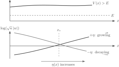
With $\eta(x)=\hbar^{-1}\int_{x_*}^{x}\kappa(s)\,ds$, the two local branches scale as $e^{+\eta}$ and $e^{-\eta}$. “Growing” and “decaying” refer to the chosen direction of increasing $\eta$, not to an intrinsic label independent of integration limits.

Boundary Conditions Select the Physical Combination

The local differential equation has two independent branches. A physical problem selects their coefficients globally.

Semi-infinite forbidden tail

Suppose the forbidden region extends to $x\to+\infty$ and

$$\eta(x)\to+\infty.$$

Normalizability requires

$$D_{\mathrm g}=0,$$

leaving

$$\psi(x) \propto \frac{e^{-\eta(x)}}{\sqrt{\kappa(x)}}.$$

This is the familiar decaying tail of a bound state. On a left-hand tail, the integral orientation must be reversed so that the selected branch decays as $x\to-\infty$.

Finite forbidden interval

Inside a finite barrier, neither local branch should be discarded before matching both ends. A solution that is small toward one edge can contain a component that grows toward the other. The coefficients are determined by the incoming, reflected, and transmitted boundary conditions after connection through both turning-point neighborhoods.

This is why the slogan “throw away the growing exponential” has limited scope. It is correct for a semi-infinite normalizable tail. It is generally wrong as a local rule inside a finite barrier.

Bound-state barrier between two wells

In a double well, the central forbidden interval connects two allowed wells. Exponentially small overlap through that interval produces even–odd level splitting. The local basis here supplies the tails; Double-Well Tunneling owns the effective two-state physics and splitting estimate.

Probability Current Under a Barrier

For a real scalar potential,

$$j = \frac{\hbar}{m} \operatorname{Im} \left( \psi^*\frac{d\psi}{dx} \right).$$

Each isolated basis function $w_{\mathrm g}$ or $w_{\mathrm d}$ is real, up to a constant overall phase. Therefore

$$j[w_{\mathrm g}] = j[w_{\mathrm d}] = 0.$$

This does not imply that every stationary state has zero current inside a forbidden region.

For

$$\psi = D_{\mathrm g}w_{\mathrm g} + D_{\mathrm d}w_{\mathrm d},$$

the Wronskian is

$$\begin{aligned} W[w_{\mathrm g},w_{\mathrm d}] &= w_{\mathrm g}w_{\mathrm d}' - w_{\mathrm g}'w_{\mathrm d} \\ &= - \frac{2}{\hbar}. \end{aligned}$$

The current is consequently

$$j_{\mathrm{WKB}} = - \frac{2}{m} \operatorname{Im} \left( D_{\mathrm g}^*D_{\mathrm d} \right).$$

A nonzero current requires both branches and a nontrivial relative complex phase. The sign shown follows the convention that $\eta$ increases with $x$ and that $w_{\mathrm g}=e^{+\eta}/\sqrt\kappa$ is listed first.

The corresponding density is

$$\begin{aligned} \lvert\psi\rvert^2 ={}& \frac{1}{\kappa} \bigg[ \lvert D_{\mathrm g}\rvert^2e^{2\eta} + \lvert D_{\mathrm d}\rvert^2e^{-2\eta} \\ &\qquad + 2\operatorname{Re} \left( D_{\mathrm g}D_{\mathrm d}^* \right) \bigg]. \end{aligned}$$

Unlike the allowed-region case, there are no spatial interference fringes between the two real exponential basis functions. Their cross term is nevertheless essential for current when the relative coefficient phase is complex.

What this means physically

• A real bound-state tail can be chosen real and has $j=0$.
• A pure decaying solution in a semi-infinite forbidden region has $j=0$.
• A stationary scattering state through a finite barrier has the same nonzero conserved current in allowed and forbidden regions.
• That under-barrier current is encoded by the complex mixture of growing and decaying local branches, not by assigning a real classical velocity to either branch.

The general current formula belongs to Probability Current. The broader physical meaning of tunneling is developed in Quantum Tunneling.

Exponential Suppression Across an Interval

For $a<b$ inside one forbidden region, define the forbidden action

$$K(a,b;E) = \int_a^b \kappa(x;E)\,dx.$$

A branch that decays toward increasing $x$ has the local amplitude ratio

$$\frac{\psi_{\mathrm d}(b)} {\psi_{\mathrm d}(a)} \approx \sqrt{ \frac{\kappa(a)}{\kappa(b)} } \exp\left[ - \frac{K(a,b;E)}{\hbar} \right].$$

Its density ratio is

$$\frac{\lvert\psi_{\mathrm d}(b)\rvert^2} {\lvert\psi_{\mathrm d}(a)\rvert^2} \approx \frac{\kappa(a)}{\kappa(b)} \exp\left[ - \frac{2K(a,b;E)}{\hbar} \right].$$

The distinction between amplitude and probability exponents is fundamental. Across an entire smooth barrier bounded by two turning points, the same action controls the leading transmission probability, but turning-point matching and flux normalization are needed before this local decay ratio becomes a scattering coefficient.

Why the Prefactor Is Not Optional

The factor $\kappa^{-1/2}$ changes slowly compared with the exponential, but it is part of leading WKB. It follows from the transport equation and is required for a controlled approximation.

For one branch,

$$\psi(x) = A(x)e^{\pm\eta(x)},$$

the leading transport equation gives

$$\frac{d}{dx} \left( \kappa A^2 \right) = 0,$$

and hence

$$A(x) \propto \frac{1}{\sqrt{\kappa(x)}}.$$

Unlike the allowed-region factor $p^{-1/2}$, this should not be interpreted as a classical dwell-time density: there is no real classical trajectory with energy $E$ in the forbidden interval. It is an analytic continuation of the semiclassical transport factor.

When $K/\hbar$ is large, the exponential often dominates an order-of-magnitude estimate. That does not make the prefactor mathematically absent. It means only that its relative influence on a logarithmic estimate is smaller.

Validity in a Forbidden Region

The forbidden-region equation is

$$\psi'' - \frac{\kappa^2}{\hbar^2}\psi = 0.$$

The common slow-variation parameter is

$$\epsilon_{\mathrm f}(x) = \left\lvert \hbar \frac{\kappa'(x)}{\kappa^2(x)} \right\rvert \ll1.$$

Since

$$\kappa' = \frac{mV'}{\kappa},$$

one may also write

$$\epsilon_{\mathrm f} = \frac{ \hbar m\lvert V'\rvert }{ \kappa^3 }.$$

Direct residual

Substituting either branch $w_{\mathrm g}$ or $w_{\mathrm d}$ gives

$$\begin{aligned} w_\pm'' - \frac{\kappa^2}{\hbar^2}w_\pm ={}& \biggl[ \frac34 \left( \frac{\kappa'}{\kappa} \right)^2 \\ &- \frac12 \frac{\kappa''}{\kappa} \biggr]w_\pm. \end{aligned}$$

A dimensionless residual is

$$\mathcal R_{\mathrm f} = \frac{\hbar^2}{\kappa^2} \left[ \frac34 \left( \frac{\kappa'}{\kappa} \right)^2 - \frac12 \frac{\kappa''}{\kappa} \right].$$

The requirement $\lvert\mathcal R_{\mathrm f}\rvert\ll1$ supplements the first-derivative test when curvature or several length scales matter.

Turning-point layer

At a simple turning point $x_t$ with forbidden side $x\gt x_t$, let

$$V(x)-E \approx F(x-x_t), \qquad F\gt0.$$

Then

$$\kappa(x) = \sqrt{2mF(x-x_t)}$$

and

$$\begin{aligned} \epsilon_{\mathrm f} &= \frac12 \left( \frac{\ell_F}{x-x_t} \right)^{3/2}, \\ \ell_F &= \left( \frac{\hbar^2}{2mF} \right)^{1/3}. \end{aligned}$$

Leading WKB requires $x-x_t\gg\ell_F$. The apparent divergence $\kappa^{-1/2}$ at $x_t$ is a breakdown of the outer approximation, not a divergence of the exact wavefunction.

Abrupt interfaces

Inside a constant forbidden plateau, the exponential solutions are exact. At an abrupt edge of that plateau, however, the slow-variation condition is not defined. Exact continuity matching, not a smooth turning-point formula, handles the interface. A rectangular barrier can therefore be an exact benchmark for the interior exponent while still lying outside smooth WKB at its boundaries.

Worked Examples

Constant forbidden plateau

Let $V(x)=V_0$ with $V_0\gt E$. Then

$$\kappa_0 = \sqrt{2m(V_0-E)}$$

is constant, and

$$\begin{aligned} \psi(x) ={}& \frac{D_{\mathrm g}}{\sqrt{\kappa_0}} e^{+\kappa_0(x-x_*)/\hbar} \\ &+ \frac{D_{\mathrm d}}{\sqrt{\kappa_0}} e^{-\kappa_0(x-x_*)/\hbar}. \end{aligned}$$

Because $\kappa_0'=\kappa_0''=0$, the WKB residual vanishes and these are exact interior solutions. For a finite rectangular barrier, the coefficients still require exact matching at both discontinuous interfaces; the local exactness of the interior basis does not make the smooth-turning-point machinery applicable there.

Linear forbidden ramp

For

$$V(x)-E = F(x-x_t), \qquad x\gt x_t,$$

the forbidden action from the turning point is

$$\begin{aligned} \eta(x) &= \frac{1}{\hbar} \int_{x_t}^{x} \sqrt{2mF(s-x_t)}\,ds \\ &= \frac{ 2\sqrt{2mF} }{ 3\hbar } (x-x_t)^{3/2}. \end{aligned}$$

The decaying outer solution is

$$\psi_{\mathrm d}(x) \propto \frac{ \exp\left[ - \dfrac{ 2\sqrt{2mF} }{ 3\hbar } (x-x_t)^{3/2} \right] }{ \bigl[2mF(x-x_t)\bigr]^{1/4} }.$$

This is the large-positive-argument asymptotic form of the decaying Airy solution, up to an overall constant. It is accurate only when $x-x_t\gg\ell_F$; the Airy function itself remains uniform through the turning point.

Harmonic-oscillator tail

For the harmonic oscillator,

$$V(x) = \frac12m\omega^2x^2,$$

write

$$E = \frac12m\omega^2a^2.$$

On the right forbidden tail $x\gt a$,

$$\kappa(x) = m\omega\sqrt{x^2-a^2}.$$

The forbidden action from the turning point is

$$\begin{aligned} K(a,x) ={}& \frac{m\omega}{2} \bigg[ x\sqrt{x^2-a^2} \\ &- a^2 \operatorname{arcosh} \left( \frac{x}{a} \right) \bigg]. \end{aligned}$$

The decaying WKB tail is

$$\psi_{\mathrm d}(x) \propto \frac{ e^{-K(a,x)/\hbar} }{ \sqrt{m\omega} \left(x^2-a^2\right)^{1/4} }.$$

For $x\gg a$,

$$\begin{aligned} \frac{K(a,x)}{\hbar} \approx{}& \frac{m\omega x^2}{2\hbar} - \frac{E}{\hbar\omega} \log\left(\frac{2x}{a}\right) \\ &- \frac{E}{2\hbar\omega}. \end{aligned}$$

For the exact oscillator energy

$$E_n = \hbar\omega \left( n+\frac12 \right),$$

the exponential contributes a power $x^{n+1/2}$ multiplying the Gaussian, while the prefactor contributes $x^{-1/2}$. Therefore

$$\psi_{\mathrm d}(x) \propto x^n \exp\left[ - \frac{m\omega x^2}{2\hbar} \right]$$

at leading large-$x$ order. This matches the exact Hermite-function tail. WKB fails near $x=a$, but far into the forbidden region it recovers both the Gaussian exponent and the polynomial power.

The exact states are developed in Quantum Harmonic Oscillator.

Practical Workflow

For a forbidden-region WKB calculation:

1. Identify each connected interval on which $V(x)-E\gt0$.
2. Define $\kappa=\sqrt{2m(V-E)}$ and state whether it is a momentum or inverse length.
3. Choose and display the limits of the forbidden action integral.
4. Label growth and decay relative to a stated direction.
5. Retain both local branches until global boundary conditions justify removing one.
6. Use normalizability to select tails of bound states.
7. Use matching at both ends for a finite barrier.
8. Distinguish an amplitude factor $e^{-K/\hbar}$ from a probability factor $e^{-2K/\hbar}$.
9. Check slow variation and the distance from every turning point or interface.
10. Benchmark the exponent, prefactor, current, or logarithmic derivative against an exact or numerical solution.

Common Mistakes

• Using $\kappa$ sometimes as momentum and sometimes as inverse length.
• Calling a branch “decaying” without stating the integral orientation.
• Discarding the growing exponential everywhere inside a finite barrier.
• Claiming that a finite-barrier scattering current vanishes because each real basis branch has zero current.
• Assigning a real classical velocity to an under-barrier exponential.
• Omitting the factor $\kappa^{-1/2}$ from the leading local solution.
• Confusing the amplitude exponent $K/\hbar$ with the probability exponent $2K/\hbar$.
• Extending the outer WKB form to $\kappa=0$.
• Applying Airy connection formulas at a discontinuous step.
• Treating a large barrier action as proof that every prefactor is irrelevant.
• Interpreting a coefficient magnitude without recording the action reference point.
• Assuming a small pointwise residual controls a tunneling observable near the barrier top.

Exercises

1. Current of a growing–decaying mixture

Let

$$\psi = D_{\mathrm g}w_{\mathrm g} + D_{\mathrm d}w_{\mathrm d},$$

where $w_{\mathrm g}$ and $w_{\mathrm d}$ are real and

$$W[w_{\mathrm g},w_{\mathrm d}] = - \frac{2}{\hbar}.$$

Show that

$$j = - \frac{2}{m} \operatorname{Im} \left( D_{\mathrm g}^*D_{\mathrm d} \right).$$

Solution

Using

$$j = \frac{\hbar}{2mi} \left( \psi^*\psi' - \psi\psi'^* \right),$$

the terms proportional to $\lvert D_{\mathrm g}\rvert^2$ and $\lvert D_{\mathrm d}\rvert^2$ cancel because the basis functions are real. The remaining terms give

$$\begin{aligned} \psi^*\psi' - \psi\psi'^* ={}& \left( D_{\mathrm g}^*D_{\mathrm d} - D_{\mathrm g}D_{\mathrm d}^* \right) \\ &\times W[w_{\mathrm g},w_{\mathrm d}]. \end{aligned}$$

Since

$$D_{\mathrm g}^*D_{\mathrm d} - D_{\mathrm g}D_{\mathrm d}^* = 2i \operatorname{Im} \left( D_{\mathrm g}^*D_{\mathrm d} \right),$$

and $W=-2/\hbar$,

$$j = - \frac{2}{m} \operatorname{Im} \left( D_{\mathrm g}^*D_{\mathrm d} \right).$$

A single branch gives zero current, while a relative complex phase can give nonzero current.

2. Semi-infinite tail

Suppose $\eta(x)\to+\infty$ as $x\to+\infty$. Which coefficient must vanish for a square-integrable state, and what current remains?

Solution

The term

$$D_{\mathrm g} \frac{e^{+\eta}}{\sqrt\kappa}$$

grows without bound, so square integrability requires $D_{\mathrm g}=0$. The remaining decaying branch can be chosen real up to an overall phase. Consequently

$$j=0.$$

This is appropriate for a stationary bound-state tail. It is not the boundary condition for a finite transmitting barrier.

3. Local decay across a constant plateau

For constant $\kappa_0$ on $a<x<b$, compute the decaying-branch amplitude and density ratios.

Solution

The forbidden action is

$$K(a,b) = \kappa_0(b-a).$$

Because the prefactor is constant,

$$\frac{\psi_{\mathrm d}(b)} {\psi_{\mathrm d}(a)} = \exp\left[ - \frac{\kappa_0(b-a)}{\hbar} \right].$$

Squaring gives

$$\frac{\lvert\psi_{\mathrm d}(b)\rvert^2} {\lvert\psi_{\mathrm d}(a)\rvert^2} = \exp\left[ - \frac{2\kappa_0(b-a)}{\hbar} \right].$$

This is a local decay ratio. A finite-barrier transmission probability additionally requires interface matching and flux normalization.

4. Linear-ramp validity

For $\kappa(x)=\sqrt{2mF(x-x_t)}$, derive

$$\epsilon_{\mathrm f} = \frac12 \left( \frac{\ell_F}{x-x_t} \right)^{3/2}.$$

Solution

Differentiate:

$$\lvert\kappa'(x)\rvert = \frac{\sqrt{2mF}}{ 2\sqrt{x-x_t} }.$$

Then

$$\begin{aligned} \epsilon_{\mathrm f} &= \hbar \frac{\lvert\kappa'\rvert}{\kappa^2} \\ &= \frac{\hbar}{ 2\sqrt{2mF} (x-x_t)^{3/2} }. \end{aligned}$$

Using

$$\ell_F^{3/2} = \frac{\hbar}{\sqrt{2mF}}$$

gives the stated result. WKB is controlled only for $x-x_t\gg\ell_F$.

5. Orientation reversal

Define

$$\eta_L(x) = \frac1\hbar \int_{x_*}^{x} \kappa(s)\,ds$$

and

$$\eta_R(x) = \frac1\hbar \int_x^{x_R} \kappa(s)\,ds.$$

Relate the two and explain why the sign attached to a decaying branch changes.

Solution

The sum

$$\eta_L(x)+\eta_R(x) = \frac1\hbar \int_{x_*}^{x_R} \kappa(s)\,ds$$

is independent of $x$. Therefore

$$e^{-\eta_L(x)} = \text{constant} \times e^{+\eta_R(x)}.$$

A function that decays as $x$ increases is written with $-\eta_L$, but with $+\eta_R$ when the action is measured backward from the right endpoint. Growth and decay are geometric properties in a chosen direction; the printed exponent sign depends on the integral convention.

6. Harmonic-oscillator tail

Use the large-$x$ form of $K(a,x)$ and $E_n=\hbar\omega(n+1/2)$ to show that the decaying WKB tail scales as

$$x^n e^{-m\omega x^2/(2\hbar)}.$$

Solution

At large $x$,

$$\begin{aligned} \frac{K(a,x)}{\hbar} \approx{}& \frac{m\omega x^2}{2\hbar} \\ &- \frac{E_n}{\hbar\omega} \log\left(\frac{2x}{a}\right) \\ &+ \text{constant}. \end{aligned}$$

Hence

$$e^{-K/\hbar} \propto e^{-m\omega x^2/(2\hbar)} x^{E_n/(\hbar\omega)}.$$

Since $E_n/(\hbar\omega)=n+1/2$, the exponential factor supplies $x^{n+1/2}$. Meanwhile

$$\kappa^{-1/2} \sim (m\omega x)^{-1/2},$$

which removes one half-power. Thus

$$\psi_{\mathrm d}(x) \propto x^n e^{-m\omega x^2/(2\hbar)}.$$

This is the large-$x$ form of a Hermite polynomial times the oscillator Gaussian.

References

1. L. D. Landau and E. M. Lifshitz, Quantum Mechanics: Non-Relativistic Theory, 3rd ed. (Butterworth-Heinemann, 1981). Forbidden-region WKB, connection formulas, and barrier penetration.
2. C. M. Bender and S. A. Orszag, Advanced Mathematical Methods for Scientists and Engineers I (Springer, 1999). Liouville–Green expansions, residuals, and turning-point asymptotics.
3. M. V. Berry and K. E. Mount, “Semiclassical approximations in wave mechanics”, Reports on Progress in Physics 35, 315–397 (1972). Phase-integral branches, barriers, and semiclassical interpretation.
4. F. W. J. Olver, Asymptotics and Special Functions (A K Peters, 1997). Error-controlled exponential and Airy asymptotics.
5. J. Heading, An Introduction to Phase-Integral Methods (Methuen, 1962). Exponential bases, Stokes structure, and connection theory.
6. R. Shankar, Principles of Quantum Mechanics, 2nd ed. (Springer, 1994). Standard WKB tunneling and bound-state examples.