Coherent-State Semiclassics Preview

Coherent-state semiclassics represents quantum evolution with states localized in phase space and then uses classical or near-classical trajectories to organize the answer. Depending on the approximation, one may propagate a single packet center, allow its covariance to evolve, solve a coherent-state boundary-value problem, or integrate over an ensemble of initial packets.

Those procedures are related, but they are not interchangeable. A single coherent state can remain exact under harmonic motion, fail immediately under a nonlinear Hamiltonian, and still serve as one element of a successful many-packet semiclassical representation.

This page is a method-selection preview. It does not repeat the canonical constructions:

• Coherent States owns the oscillator definition, number expansion, displacement operator, and minimum-uncertainty formulas.
• Coherent States in Phase Space owns the Wigner-function geometry.
• Coherent-State Dynamics owns exact harmonic and driven evolution.
• Time-Dependent Variational Principle owns tangent-space projection and residual error control.
• Spin Coherent States owns the spherical phase space and large-spin construction.

The purpose here is to explain what a coherent-state semiclassical calculation approximates, which trajectory equations it uses, and where its phase, prefactor, or state-manifold assumptions fail.

Minimal Phase-Space Recap

For one canonical degree of freedom, choose a positive width scale $b$ and define

$$z = \frac{1}{\sqrt{2}} \left( \frac{q}{b} + i\frac{bp}{\hbar} \right).$$

The corresponding normalized oscillator coherent states satisfy

$$\hat a\lvert z\rangle = z\lvert z\rangle$$

and resolve the identity:

$$I = \int_{\mathbb C} \frac{d^2z}{\pi} \lvert z\rangle \langle z\rvert.$$

Their overlap is

$$\langle z'\vert z\rangle = \exp\left[ \begin{gathered} -\dfrac{\lvert z'\rvert^2}{2} -\dfrac{\lvert z\rvert^2}{2} \\ +z'^*z \end{gathered} \right],$$

so

$$\lvert\langle z'\vert z\rangle\rvert^2 = e^{-\lvert z'-z\rvert^2}.$$

The states are localized but nonorthogonal. Their canonical variances are

$$\Delta q = \frac{b}{\sqrt2}, \qquad \Delta p = \frac{\hbar}{\sqrt2\,b},$$

and therefore

$$\Delta q\,\Delta p = \frac{\hbar}{2}.$$

The freedom to choose $b$ is part of the approximation whenever the Hamiltonian does not select a natural oscillator width. A poor width can make a frozen packet inefficient even when a broader Gaussian or many-packet method works well.

The Semiclassical Scaling

In a standard canonical limit, hold the physical phase-space center $(q,p)$ fixed while taking

$$b = O(\sqrt{\hbar}).$$

Then

$$\Delta q = O(\sqrt{\hbar}), \qquad \Delta p = O(\sqrt{\hbar}),$$

while

$$\lvert z\rvert^2 = O(\hbar^{-1})$$

away from the phase-space origin. The packet occupies a shrinking phase-space neighborhood even though its coherent-state label becomes large.

At fixed $\hbar$, large occupation can provide a related limit. For a canonical coherent state,

$$\langle N\rangle = \lvert z\rvert^2, \qquad \frac{\Delta N}{\langle N\rangle} = \frac{1}{\sqrt{\langle N\rangle}}.$$

Small relative number fluctuations help explain classical-looking field amplitudes, but they do not imply zero absolute noise, exact orthogonality, or immunity to nonlinear quantum evolution.

Three Different Approximations

The phrase “propagate a coherent state semiclassically” can refer to three distinct levels.

Exact invariant motion

For a Hamiltonian that is at most a phase rotation and displacement in $\hat a$ and $\hat a^\dagger$, an initial coherent state remains in the coherent-state family:

$$e^{-i\hat Ht/\hbar} \lvert z_0\rangle = e^{i\chi(t)} \lvert z(t)\rangle.$$

The packet center follows a classical affine symplectic trajectory, its covariance remains the coherent-state covariance, and only the state-vector phase requires additional bookkeeping. This is exact quantum dynamics, not merely a leading semiclassical estimate.

One projected packet

For a generic Hamiltonian, impose an ansatz

$$\lvert\psi(t)\rangle \approx e^{i\chi(t)} \lvert z(t)\rangle$$

and determine $z(t)$ variationally. This projects the Schrödinger velocity onto the tangent space of the coherent-state manifold. The result can track a packet center while missing squeezing, spreading, skewness, splitting, or interference.

Allowing a time-dependent covariance produces a thawed Gaussian manifold. It is larger than the ordinary coherent-state family and is exact for general quadratic Hamiltonians when the phase and width equations are treated consistently.

A trajectory sum

Instead of claiming that the state remains one packet, represent a propagator or wavefunction as a coherent sum over many trajectory contributions:

$$\mathcal A_{\mathrm{sc}} \sim \sum_\gamma \mathcal C_\gamma^{1/2} e^{iS_\gamma/\hbar+i\Delta_\gamma}.$$

The labels $\gamma$ may denote coherent-state boundary-value saddles or trajectories launched from initial phase-space points. The prefactor $\mathcal C_\gamma$ carries stability information, and $\Delta_\gamma$ includes convention-dependent phase corrections.

This level can represent deformation and interference even when every basis packet is frozen, because the total state is a superposition of many packets.

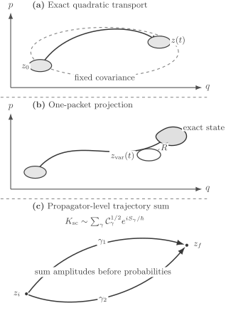
Top: quadratic dynamics can transport a coherent packet exactly with fixed covariance. Middle: a nonlinear flow deforms the exact state, while a one-packet variational trajectory remains on the chosen manifold and leaves a residual. Bottom: a propagator-level approximation sums several trajectory amplitudes and can retain interference.

Variational Phase-Space Dynamics

For normalized canonical coherent states, define the covariant or $Q$ symbol

$$H_Q(z^*,z) = \langle z\vert \hat H \vert z\rangle.$$

Restricting the quantum action to the coherent-state manifold gives

$$\begin{aligned} S_{\mathrm{var}} ={}& \int_{t_i}^{t_f}dt \Bigg[ \frac{i\hbar}{2} \left( z^*\dot z - \dot z^*z \right) \\ &\qquad\qquad - H_Q(z^*,z) \Bigg]. \end{aligned}$$

Stationary variation yields

$$i\hbar\dot z = \frac{\partial H_Q}{\partial z^*},$$

and its conjugate equation when the trajectory remains on the real phase-space section. In $(q,p)$ coordinates these are Hamilton equations generated by the restricted energy $H_Q(q,p)$.

This classical-looking form does not make the approximation exact. It only states that the chosen variational manifold inherits a symplectic structure.

Which Hamiltonian function appears?

For

$$\hat H = \frac{\hat p^2}{2m} + V(\hat q),$$

a smooth-potential expansion around the coherent-state center gives

$$\begin{aligned} H_Q(q,p) ={}& \frac{p^2}{2m} + \frac{\hbar^2}{4mb^2} + V(q) \\ &+ \frac{b^2}{4}V''(q) + O\left( b^4V^{(4)} \right). \end{aligned}$$

If $b^2=O(\hbar)$, the difference between $H_Q$ and the point-particle Hamiltonian begins at order $\hbar$. Such corrections may be small in the trajectory equations yet still contribute an order-one phase after division by $\hbar$.

Different coherent-state symbols, including normal, antinormal, and Weyl symbols, differ by terms of this type. A calculation must state which symbol and time-slicing convention it uses.

Residual as the decisive test

For an optimally phased variational state, define

$$\lvert R(t)\rangle = \left( i\hbar\frac{d}{dt} - \hat H \right) \lvert\psi_{\mathrm{var}}(t)\rangle.$$

If $R=0$, the variational manifold is invariant along the trajectory and the motion is exact. If $R\ne0$, the discarded component drives the state out of the manifold. The integrated scale

$$\frac{1}{\hbar} \int_0^T \lVert R(t)\rVert\,dt$$

is an a posteriori diagnostic for accumulated state error. The precise projection and error bound belong to the canonical Time-Dependent Variational Principle page.

Frozen and Thawed Gaussians

A frozen Gaussian keeps its covariance fixed while its center and phase evolve. An ordinary canonical coherent state is a frozen Gaussian.

A thawed Gaussian also evolves a complex width or covariance matrix. Linearized classical stability then controls squeezing, rotation, and spreading. For a quadratic Hamiltonian, the thawed Gaussian family is invariant and reproduces exact Gaussian evolution.

For a nonlinear potential, expand around the packet center:

$$\begin{aligned} V(q+\xi) ={}& V(q) + V'(q)\xi + \frac12V''(q)\xi^2 \\ &+ \frac{1}{6}V'''(q)\xi^3 + \cdots. \end{aligned}$$

The constant, linear, and quadratic terms preserve Gaussianity. Cubic and higher terms generate non-Gaussian structure. A thawed packet can delay failure by following the local curvature, but it cannot represent arbitrary skewness, splitting, or interference with one Gaussian.

This distinction prevents a common confusion:

• one frozen Gaussian cannot spread;
• a superposition or integral of many frozen Gaussians can spread and deform through changing centers, prefactors, and interference.

Coherent-State Propagator

The canonical coherent-state propagator is

$$K(z_f^*,z_i;T) = \langle z_f\vert e^{-i\hat HT/\hbar} \vert z_i\rangle.$$

The notation emphasizes that a Bargmann-space propagator is holomorphic in the initial label $z_i$ and antiholomorphic in the final label $z_f^*$ after the standard normalization factors are separated.

Repeated insertion of the coherent-state resolution of identity gives a time-sliced phase-space path integral. A continuum action is often written schematically as

$$\begin{aligned} \mathcal S[v,u] ={}& \int_0^Tdt \Bigg[ \frac{i\hbar}{2} \left( v\dot u - \dot v u \right) \\ &\qquad\qquad - H_{\mathrm{symb}}(v,u) \Bigg] + \mathcal B, \end{aligned}$$

where $\mathcal B$ is an endpoint term fixed by the discretization and normalization convention.

Mixed boundary data

The saddle equations are first order:

$$i\hbar\dot u = \frac{\partial H_{\mathrm{symb}}}{\partial v}, \qquad - i\hbar\dot v = \frac{\partial H_{\mathrm{symb}}}{\partial u}.$$

For the propagator above, the natural boundary data are mixed:

$$u(0)=z_i, \qquad v(T)=z_f^*.$$

One does not generally fix both $u$ and $v$ at both endpoints. Along a complex saddle, $u(t)$ and $v(t)$ are independent complex variables; $v(t)$ need not equal $u(t)^*$ between the endpoints.

This is one reason coherent-state semiclassical propagation is not merely “follow the real classical orbit from $z_i$ to $z_f$.”

Saddle sum and stability

At leading semiclassical order,

$$K_{\mathrm{sc}} \sim \sum_\gamma \mathcal C_\gamma^{1/2} \exp\left[ \frac{i}{\hbar} \mathcal S_\gamma + i\Delta_\gamma \right].$$

The sum runs over relevant saddles satisfying the mixed endpoint data. The factor $\mathcal C_\gamma$ is built from the linearized map between endpoint variations, in close analogy with the Van Vleck Determinant.

The correction $\Delta_\gamma$ depends on the coherent-state family, Hamiltonian symbol, and discretization. In common spin and bosonic conventions it includes a Solari–Kochetov-type phase. Because an order-$\hbar$ shift in the action produces an order-one shift in $\mathcal S/\hbar$, this correction matters for phase-accurate interference.

Phase-space caustics

The coherent-state prefactor becomes singular when the relevant endpoint map loses local invertibility. This is a phase-space caustic, not a divergence of the exact propagator.

Near such a point:

• two or more saddles may coalesce;
• isolated Gaussian saddle terms cease to be uniform;
• a representation change or uniform approximation is required;
• branch and phase bookkeeping becomes essential.

The logic is the same as at WKB turning points and configuration-space caustics, although the singular map and canonical integral depend on the representation.

Initial-Value Representations

Boundary-value coherent-state saddles can require a difficult search for complex trajectories. An initial-value representation, or IVR, instead integrates over real initial phase-space points and propagates each point forward.

A frozen-Gaussian IVR has the schematic operator form

$$\begin{aligned} \hat U_{\mathrm{IVR}}(t) \sim{}& \int \frac{d^nq_0\,d^np_0} {(2\pi\hbar)^n} \, C_t(q_0,p_0) \\ &\times e^{iS_t(q_0,p_0)/\hbar} \lvert g_{q_t,p_t}\rangle \langle g_{q_0,p_0}\rvert. \end{aligned}$$

Here $(q_t,p_t)$ is the classical trajectory launched from $(q_0,p_0)$, $S_t$ is its action, and $C_t$ depends on the stability matrix and packet width. The Herman–Kluk propagator is the best-known example.

An IVR replaces trajectory root searches with an oscillatory phase-space integral. That trade is useful but not free:

• the stability prefactor may grow or fluctuate strongly;
• destructive interference causes a sampling or sign problem;
• chaotic dynamics can make long-time convergence difficult;
• width choices affect numerical efficiency;
• approximate propagation need not be exactly unitary;
• tunneling may require complexification or additional treatment.

The IVR is a trajectory-sum approximation. It should not be confused with a single frozen packet following one orbit.

Worked Contrast: Harmonic and Kerr Evolution

For the harmonic oscillator,

$$\hat H_0 = \hbar\omega \left( \hat N+\frac12 \right),$$

the number-state phases are linear in $n$. The coherent-state expansion therefore reorganizes into another coherent state:

$$e^{-i\hat H_0t/\hbar} \lvert z_0\rangle = e^{-i\omega t/2} \lvert z_0e^{-i\omega t}\rangle.$$

Now add a Kerr-type nonlinearity:

$$\hat H_K = \hbar\omega\hat N + \frac{\hbar\chi}{2} \hat N(\hat N-1).$$

Exact evolution gives

$$\lvert\psi(t)\rangle = e^{-\lvert z_0\rvert^2/2} \sum_{n=0}^{\infty} c_n(t) \lvert n\rangle.$$

Here

$$c_n(t) = \frac{z_0^n}{\sqrt{n!}} e^{-it\Omega_n},$$

with

$$\Omega_n = \omega n + \frac{\chi}{2}n(n-1).$$

The phase is quadratic in $n$, so the coefficients cannot generally be written as one global phase times $z(t)^n$. The state shears, collapses, revives, and can form nonclassical superpositions.

A coherent-state variational trajectory may still approximate the center for a limited time. It does not reproduce the full state once the number-dependent phase varies appreciably across the occupied range

$$\Delta n \sim \lvert z_0\rvert.$$

This example cleanly separates classical-looking centroid motion from accurate quantum-state propagation.

Spin and Generalized Coherent States

Coherent-state semiclassics is not confined to the oscillator plane.

Family	Classical phase space	Semiclassical scale	Canonical home
Canonical oscillator states	plane	action over $\hbar$ or large occupation	Coherent States
Spin coherent states	sphere	large-$s$ limit	Spin Coherent States
Bosonic multimode states	product of mode planes	large mode occupations or field action	Harmonic Oscillator to Fields

For a spin coherent state $\lvert\hat{\mathbf n};s\rangle$, the phase-space action contains a Berry term:

$$\begin{aligned} S[\theta,\phi] = \int dt \Big[ \hbar s (1-\cos\theta)\dot\phi \\ - H_Q(\theta,\phi) \Big]. \end{aligned}$$

The sphere, its symplectic area, and the large-$s$ fluctuation scaling replace the oscillator plane and large occupation. The local Berry connection depends on a gauge patch, while closed-loop physical phases depend on the enclosed solid angle.

Generalized coherent states share localization, overcompleteness, and group-orbit geometry, but their measures, symbols, curvatures, and semiclassical corrections are family-specific.

Quantum Optics and QFT Boundary

For retained bosonic modes,

$$\hat a_{\mathbf k} \lvert\{\alpha\}\rangle = \alpha_{\mathbf k} \lvert\{\alpha\}\rangle.$$

Under a free or linearly driven field Hamiltonian, the mode amplitudes obey the corresponding classical linear equations, and a product coherent state remains coherent. This underlies the use of coherent states for idealized laser fields and classical radiation.

Several boundaries must remain explicit:

• a coherent state retains vacuum and shot-noise fluctuations;
• large occupation suppresses relative fluctuations, not all quantum effects;
• interactions can squeeze modes, entangle them, and generate non-Gaussian correlations;
• a coherent-state path-integral variable is an integration label, not proof that the exact state stays coherent;
• continuum QFT requires regularization and renormalization;
• gauge fields require constraints, gauge fixing, or a physical-mode construction;
• inequivalent representations and infrared issues can arise with infinitely many modes.

The finite-mode oscillator picture is therefore a bridge, not a substitute for field-theoretic analysis. See Path Integrals and Harmonic Oscillator to Fields.

Method-Selection Workflow

1. Define the coherent family

State the labels, measure, overlap convention, width or covariance, and whether the states are canonical, squeezed, spin, or another generalized family.

2. Identify the control parameter

Examples include action over $\hbar$, large occupation, large spin, a narrow packet scale, or weak nonlinearity over the propagation time.

3. Choose the approximation level

Use exact coherent motion only for an invariant family. Use TDVP for a projected single-manifold trajectory. Use a thawed Gaussian when covariance dynamics matters. Use a coherent-state propagator or IVR when multiple trajectories and interference are essential.

4. Fix symbols and endpoints

For a path integral, declare the time slicing, Hamiltonian symbol, endpoint term, mixed boundary data, and contour or complex-saddle prescription.

5. Propagate stability data

Trajectory centers alone do not determine a semiclassical amplitude. Propagate the monodromy matrix, Gaussian width, determinant branch, and phase correction required by the chosen method.

6. Sum amplitudes coherently

Different saddles or initial packets interfere. Do not replace their sum by a probability mixture unless a separate decoherence or coarse-graining argument justifies it.

7. Validate

Compare with exact quadratic benchmarks, residual norms, width enlargement, trajectory and sampling convergence, norm or unitarity drift, and direct quantum propagation where feasible.

Failure Diagnostics

• Packet deformation: covariance growth or non-Gaussian cumulants show that one coherent state is insufficient.
• Branching and interference: one trajectory cannot represent separated wave-packet branches.
• Caustics: a singular stability prefactor requires a uniform repair or representation change.
• Long-time instability: chaotic stretching can defeat a locally valid short-time approximation.
• Symbol ambiguity: inconsistent ordering and time slicing produce wrong order-one phases.
• Boundary overspecification: fixing both complex variables at both endpoints generally gives the wrong saddle problem.
• Complex dynamics: tunneling and forbidden transitions may require complex saddles.
• Sampling failure: an IVR integral can be dominated by cancellations that are numerically hard to resolve.
• False classicality: localized states and classical centroids do not imply decoherence or a classical probability theory.

Which Canonical Page to Use

Need	Canonical page
Oscillator coherent-state construction	Coherent States
Exact harmonic and driven evolution	Coherent-State Dynamics
Wigner-function localization	Coherent States in Phase Space
Berry geometry and many-body field actions	Coherent-State Path Integrals
Variational projection and residual bounds	Time-Dependent Variational Principle
General saddle-point method	Stationary Phase in Quantum Mechanics
Configuration-space trajectory propagator	Semiclassical Propagator
Stability determinants	Van Vleck Determinant
Spin coherent states and spherical phase space	Spin Coherent States
Oscillator-to-field dictionary	Harmonic Oscillator to Fields

Common Mistakes

• Treating every localized Gaussian as a coherent state of the chosen oscillator.
• Assuming that classical centroid motion makes the full quantum state classical.
• Calling a TDVP trajectory exact without checking invariance or the residual.
• Expecting one frozen packet to spread or split.
• Forgetting that a sum of frozen packets can nevertheless deform and interfere.
• Using the point-particle Hamiltonian when the chosen method requires a specified coherent-state symbol.
• Dropping order-$\hbar$ symbol corrections even when phase accuracy is required.
• Setting $v=u^*$ on a complex coherent-state saddle without justification.
• Overspecifying first-order coherent-state boundary equations.
• Ignoring determinant branches, phase-space caustics, or Solari–Kochetov-type phases.
• Assuming a large occupation number eliminates shot noise, squeezing, or entanglement.
• Treating an IVR as automatically unitary or convergent at long times.

Exercises

1. Phase-space distance and overlap

Using

$$z = \frac{1}{\sqrt2} \left( \frac{q}{b} + i\frac{bp}{\hbar} \right),$$

express

$$\lvert\langle z'\vert z\rangle\rvert^2$$

in terms of $\Delta q=q'-q$ and $\Delta p=p'-p$.

Solution

The label separation is

$$z'-z = \frac{1}{\sqrt2} \left( \frac{\Delta q}{b} + i\frac{b\Delta p}{\hbar} \right).$$

Therefore

$$\lvert z'-z\rvert^2 = \frac{(\Delta q)^2}{2b^2} + \frac{b^2(\Delta p)^2}{2\hbar^2}.$$

Using the canonical overlap,

$$\boxed{ \lvert\langle z'\vert z\rangle\rvert^2 = \exp\left[ - \frac{(\Delta q)^2}{2b^2} - \frac{b^2(\Delta p)^2}{2\hbar^2} \right] }.$$

The overlap falls when the centers are separated by more than the packet resolution in either quadrature. It never vanishes exactly at finite separation.

2. Harmonic variational trajectory

For

$$H_Q(z^*,z) = \hbar\omega \left( z^*z+\frac12 \right),$$

derive the coherent-state equation of motion and solve it.

Solution

The variational equation is

$$i\hbar\dot z = \frac{\partial H_Q}{\partial z^*} = \hbar\omega z.$$

Hence

$$\dot z = - i\omega z,$$

with solution

$$z(t) = z(0)e^{-i\omega t}.$$

For the harmonic oscillator this is not merely variational: the coherent-state family is invariant, so the state remains coherent after the overall phase is included.

3. Why the endpoint data are mixed

Vary

$$\begin{aligned} \mathcal S[v,u] ={}& \int_0^Tdt \frac{i\hbar}{2} \left( v\dot u-\dot v u \right) \\ &- \int_0^Tdt\, H(v,u) + \mathcal B \end{aligned}$$

and explain why a coherent-state propagator naturally fixes $u(0)$ and $v(T)$ rather than both variables at both times.

Solution

Integrating the kinetic variation by parts gives a bulk term

$$\begin{aligned} \delta\mathcal S_{\mathrm{bulk}} ={}& \int_0^Tdt \Bigg[ \left( i\hbar\dot u - \frac{\partial H}{\partial v} \right)\delta v \\ &+ \left( - i\hbar\dot v - \frac{\partial H}{\partial u} \right)\delta u \Bigg], \end{aligned}$$

plus endpoint terms. The convention-dependent $\mathcal B$ is chosen so that the remaining endpoint variation vanishes when

$$\delta u(0)=0, \qquad \delta v(T)=0.$$

The bulk equations are first order in time. Fixing $u(0)$ and $v(T)$ supplies the required mixed data. Fixing both $u$ and $v$ at both endpoints would generally overdetermine the saddle equations.

4. An order-one phase from an order-ℏ symbol shift

Suppose two consistent Hamiltonian symbols differ by

$$H_2 = H_1 + \hbar h_1.$$

For a fixed trajectory and propagation time, find the resulting difference in the dynamical exponent.

Solution

The action difference from the Hamiltonian term is

$$\Delta S = - \hbar \int_0^T h_1(t)\,dt.$$

Dividing by $\hbar$ gives

$$\frac{\Delta S}{\hbar} = - \int_0^T h_1(t)\,dt.$$

Thus an order-$\hbar$ symbol difference changes the semiclassical phase by order unity. Symbol and discretization corrections can be subleading in the trajectory while remaining leading for interference phases.

5. Kerr evolution leaves the coherent manifold

For the Kerr Hamiltonian in the worked contrast, show that the evolved state cannot generally equal

$$e^{i\chi(t)} \lvert z(t)\rangle.$$

Solution

If the state remained coherent, the ratio of adjacent number-basis coefficients would be

$$\frac{c_{n+1}(t)}{c_n(t)} = \frac{z(t)}{\sqrt{n+1}},$$

apart from one global phase. Exact Kerr evolution instead gives

$$\begin{aligned} \frac{c_{n+1}(t)}{c_n(t)} ={}& \frac{z_0}{\sqrt{n+1}} \\ &\times \exp\left[ - it \left( \omega+\chi n \right) \right]. \end{aligned}$$

The extra factor depends on $n$ when $\chi t$ is not an integer multiple of $2\pi$. No single label $z(t)$ can reproduce all adjacent ratios. The state has left the ordinary coherent-state manifold.

6. One frozen packet versus a frozen-packet IVR

Explain how a frozen-Gaussian IVR can describe a changing total wave-packet width even though each basis packet keeps a fixed covariance.

Solution

An IVR constructs the state from a continuum of packets:

$$\lvert\psi(t)\rangle \sim \int d\Gamma_0\, A_t(\Gamma_0) \lvert g_{\Gamma_t}\rangle,$$

where $\Gamma_t$ is the classically propagated center and $A_t$ contains phases and stability factors.

Different centers separate, focus, and interfere as time evolves. The envelope and covariance of the sum therefore change even though the covariance of each individual $\lvert g_{\Gamma_t}\rangle$ is fixed. A single frozen packet lacks this mechanism; a coherent superposition of many frozen packets does not.

References

1. R. J. Glauber, “Coherent and incoherent states of the radiation field”, Physical Review 131, 2766–2788 (1963). Canonical field-mode coherent states and optical coherence.
2. G. A. Hagedorn, “Semiclassical quantum mechanics. I. The $\hbar\to0$ limit for coherent states”, Communications in Mathematical Physics 71, 77–93 (1980). Controlled coherent-state propagation in the semiclassical limit.
3. E. J. Heller, “Time-dependent approach to semiclassical dynamics”, Journal of Chemical Physics 62, 1544–1555 (1975). Gaussian wave-packet dynamics and local quadratic propagation.
4. M. F. Herman and E. Kluk, “A semiclasical justification for the use of non-spreading wavepackets in dynamics calculations”, Chemical Physics 91, 27–34 (1984). Frozen-Gaussian initial-value representation.
5. M. Baranger, M. A. M. de Aguiar, F. Keck, H. J. Korsch, and B. Schellhaass, “Semiclassical approximations in phase space with coherent states”, Journal of Physics A 34, 7227–7286 (2001). Coherent-state propagators, symbols, complex trajectories, and phase-space caustics.
6. H. G. Solari, “Semiclassical treatment of spin system by means of coherent states”, Journal of Mathematical Physics 28, 1097–1102 (1987). Discretization-sensitive phase correction.
7. E. A. Kochetov, “SU(2) coherent-state path integral for the Heisenberg ferromagnet”, Physical Review B 52, 4402–4408 (1995). Spin coherent-state semiclassics and extra-phase structure.
8. M. Stone, K.-S. Park, and A. Garg, “The semiclassical propagator for spin coherent states”, Journal of Mathematical Physics 41, 8025–8049 (2000). Fluctuation determinants and the Solari–Kochetov correction.
9. J. R. Klauder and B.-S. Skagerstam, eds., Coherent States: Applications in Physics and Mathematical Physics (World Scientific, 1985). Generalized coherent states and path-integral methods.
10. A. Perelomov, Generalized Coherent States and Their Applications (Springer, 1986). Group-orbit coherent states and geometry.