Coherent-State Path Integrals

A coherent-state path integral rewrites operator evolution using an overcomplete family of states rather than an orthogonal coordinate basis. Its distinctive first-order term is not guessed from a classical field equation. It comes from the phase of adjacent coherent-state overlaps.

At finite slice number, a transition amplitude has the skeleton

$$\begin{aligned} K &= \int \prod_{j=1}^{M-1} d\mu(\xi_j) \\ &\quad\times \prod_{j=0}^{M-1} \langle\xi_{j+1}| e^{-i\epsilon H/\hbar} |\xi_j\rangle. \end{aligned}$$

The short-time Hamiltonian matrix element supplies an operator symbol. The overlap $\langle\xi_{j+1}|\xi_j\rangle$ supplies a measure, a phase, and the correct endpoint structure. Only after preserving all four pieces may one use the compact continuum action

$$S[\xi] = \int dt\, \left[ \mathcal A_i(\xi)\dot\xi^i - H_\sigma(\xi) \right].$$

Here $\mathcal A$ is a Berry one-form and $H_\sigma$ is the Hamiltonian symbol selected by the slicing convention. The notation is geometric, but the construction remains anchored to a regulated Hilbert-space amplitude.

Canonical Scope

This page is the canonical bridge for:

• deriving the coherent-state Berry one-form from neighboring overlaps;
• reading its curvature as the symplectic form of the coherent-state manifold;
• comparing the canonical bosonic plane with the spin coherent-state sphere;
• understanding first-order actions, mixed endpoint data, and boundary terms;
• translating bosonic amplitudes into number–phase and density–phase variables;
• identifying what survives when mode labels become spatial fields;
• distinguishing the bosonic geometry from the graded fermionic construction;
• locating ordering, gauge-patch, semiclassical, and continuum hazards.

Neighboring pages retain separate ownership:

• Coherent-State Path Integrals Preview owns finite-slice bosonic and fermionic thermal traces, Berezin integration, periodicity, antiperiodicity, free determinants, and detailed ordering benchmarks.
• Coherent-State Semiclassics Preview owns saddle sums, stability matrices, caustics, initial-value representations, and Solari–Kochetov-type corrections.
• Spin Coherent States owns the state construction, overlap, resolution of identity, and the distinction between the coherent-state sphere and the full pure-state space.
• From Berry Phase to Topological Terms owns the wider taxonomy of theta, Wess–Zumino, winding, and Chern–Simons terms.
• Nonrelativistic Field Theory from Many-Body QM owns continuum operator fields, conserved number current, contact matching, and the nonrelativistic effective-field-theory limit.

The goal here is not to replace those derivations. It is to expose the common geometric mechanism connecting Fock-space overlaps to field-theory actions.

Keep the Finite-Slice Definition

Continuum coherent-state notation suppresses data that can change the answer. A trustworthy calculation first records:

1. the Hilbert space and coherent-state family;
2. normalization and the resolution of identity;
3. the finite time lattice and direction of adjacent overlaps;
4. the operator symbol evaluated on adjacent slices;
5. endpoint or thermal closure conditions;
6. the limiting procedure used to remove the time lattice.

For a single bosonic mode, for example, the short-time ratio

$$\frac{ \langle z_{j+1}| e^{-i\epsilon H/\hbar} |z_j\rangle }{ \langle z_{j+1}|z_j\rangle }$$

is the primary object. Replacing it immediately by an arbitrary diagonal function of one smooth variable can lose ordering constants and endpoint terms. A continuum action is shorthand for a specified limit, not an independent definition.

Geometry from Overlaps

Let $|\xi\rangle$ be a smooth normalized coherent-state family. Its local Berry one-form is

$$\mathcal A = i\hbar \langle\xi|d\xi\rangle.$$

Normalization implies that $\langle\xi|d\xi\rangle$ is purely imaginary, so $\mathcal A$ is real on an ordinary real parameter manifold. Its curvature is

$$\Omega = d\mathcal A.$$

The phase convention of the state is a gauge choice. Under

$$|\xi\rangle \longmapsto e^{i\chi(\xi)}|\xi\rangle,$$

the one-form changes as

$$\mathcal A \longmapsto \mathcal A - \hbar\,d\chi,$$

while $\Omega$ is unchanged. For a closed path $C$ contained in a valid gauge patch,

$$\exp\left( \frac{i}{\hbar} \oint_C\mathcal A \right)$$

is invariant under single-valued gauge changes. If $C=\partial\Sigma$, then

$$\oint_C\mathcal A = \int_\Sigma\Omega$$

whenever one patch covers the chosen surface. Multiple patches require transition functions, as the spin sphere will illustrate.

The overlap gives an operational derivation. For nearby normalized states,

$$\langle\xi+d\xi|\xi\rangle = \exp\left[ -\langle\xi|d\xi\rangle + \mathcal O(d\xi^2) \right].$$

Multiplying these phases along the discretized path produces the line integral of $\mathcal A$. The quadratic part of the overlap controls the local metric and short-step suppression. Phase and magnitude are therefore two aspects of the same overlap kernel.

The Canonical Bosonic Plane

For one oscillator mode, use normalized coherent states

$$|z\rangle = e^{-|z|^2/2} e^{z a^\dagger}|0\rangle, \qquad a|z\rangle = z|z\rangle.$$

Their overlap and identity resolution are

$$\begin{aligned} \langle z'|z\rangle &= \exp\left[ -\frac{|z'|^2}{2} -\frac{|z|^2}{2} +\bar z'z \right], \\ I &= \int\frac{d^2z}{\pi} |z\rangle\langle z|. \end{aligned}$$

Differentiating the overlap gives

$$\mathcal A_{\mathrm B} = \frac{i\hbar}{2} \left( \bar z\,dz - z\,d\bar z \right),$$

and hence

$$\Omega_{\mathrm B} = i\hbar\, d\bar z\wedge dz.$$

Introduce real canonical coordinates through

$$z = \frac{q+ip}{\sqrt{2\hbar}}.$$

Then

$$\begin{aligned} \mathcal A_{\mathrm B} &= \frac12 \left( p\,dq-q\,dp \right), \\ \Omega_{\mathrm B} &= dp\wedge dq. \end{aligned}$$

This differs from the common canonical potential $p\,dq$ by a total derivative. Both produce the same curvature and bulk Hamilton equations, but their endpoint terms differ.

Geometry Ledger

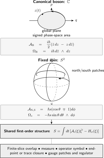
Adjacent overlaps generate a local one-form $\mathcal A$. Its curvature $\Omega=d\mathcal A$ is the symplectic form. The canonical bosonic family lives on a complex plane, whereas a fixed-spin coherent family lives on a two-patch sphere. The same first-order action is meaningful only together with its measure, symbol, endpoints, and regulator.

Symmetric and Holomorphic Actions

The normalized-state Berry form leads to the symmetric real-time kinetic term

$$S_{\mathrm B} = \int_0^T dt\, \left[ \frac{i\hbar}{2} \left( \bar z\dot z - \dot{\bar z}z \right) - H_\sigma(\bar z,z) \right].$$

Many-body calculations often use the holomorphic form

$$S_{\mathrm{hol}} = \int_0^T dt\, \left[ i\hbar\bar z\dot z - H_\sigma(\bar z,z) \right] + S_\partial.$$

The two bulk kinetic terms obey

$$\begin{aligned} i\hbar\bar z\dot z &= \frac{i\hbar}{2} \left( \bar z\dot z - \dot{\bar z}z \right) \\ &\quad+ \frac{i\hbar}{2} \frac{d}{dt} (\bar z z). \end{aligned}$$

The total derivative vanishes for a smooth closed path, but not for an open propagator. It must be combined with the coherent-state normalization and the boundary term inherited from the finite-slice product.

The bulk equations are first order:

$$\begin{aligned} i\hbar\dot z &= \frac{\partial H_\sigma}{\partial\bar z}, \\ -i\hbar\dot{\bar z} &= \frac{\partial H_\sigma}{\partial z}. \end{aligned}$$

On a real classical trajectory $\bar z=z^*$, but a saddle satisfying mixed coherent-state endpoint data can be genuinely complex.

Mixed Endpoint Data

Consider the Bargmann kernel

$$K(\bar z_f,z_i;T) = (z_f| e^{-iHT/\hbar} |z_i),$$

where $|z)=e^{za^\dagger}|0\rangle$ is unnormalized. One useful action convention is

$$\begin{aligned} \mathcal S_{\mathrm{hol}} &= -i\hbar\bar z_f z(T) \\ &\quad+ \int_0^Tdt\, \left[ i\hbar\bar z\dot z - H_\sigma(\bar z,z) \right]. \end{aligned}$$

The variational problem fixes

$$z(0)=z_i, \qquad \bar z(T)=\bar z_f.$$

It does not fix $\bar z(0)$ or $z(T)$. Varying the endpoint term cancels the remaining variation at $T$. Other normalizations distribute endpoint terms differently, but the finite-slice kernel fixes the complete answer.

This mixed boundary problem is the coherent-state analogue of fixing the initial coordinate and final conjugate coordinate. Imposing both $z$ and $\bar z$ at both ends generally overdetermines the first-order equations.

Euclidean Continuation

Under $t=-i\tau$, the real-time weight becomes a Euclidean weight,

$$e^{iS/\hbar} \longmapsto e^{-S_{\mathrm E}/\hbar}.$$

For a normal-ordered bosonic thermal generator $\mathcal K=H-\mu N$, the common holomorphic shorthand is

$$S_{\mathrm E} = \int_0^{\beta\hbar} d\tau\, \left[ \hbar\bar z\partial_\tau z + \mathcal K_{\mathrm N}(\bar z,z) \right],$$

with periodic closure for bosons. The symmetric Euclidean kinetic term is

$$\frac{\hbar}{2} \left( \bar z\partial_\tau z - (\partial_\tau\bar z)z \right).$$

For a smooth periodic path the difference is a total derivative. At finite slice number or with open endpoints, that observation does not license discarding the boundary data. The thermal trace derivation and its convergence conditions remain in Coherent-State Path Integrals Preview.

Number–Phase Variables

Write a nonzero bosonic amplitude as

$$z = \sqrt n\,e^{-i\theta}.$$

Then

$$\mathcal A_{\mathrm B} = \hbar n\,d\theta, \qquad \Omega_{\mathrm B} = \hbar\,dn\wedge d\theta.$$

The action becomes

$$S = \int dt\, \left[ \hbar n\dot\theta - H_\sigma(n,\theta) \right],$$

so the equations are

$$\begin{aligned} \hbar\dot\theta &= \frac{\partial H_\sigma}{\partial n}, \\ \hbar\dot n &= - \frac{\partial H_\sigma}{\partial\theta}. \end{aligned}$$

Thus $\hbar n$ is conjugate to $\theta$. The phase is undefined at $n=0$, so polar variables do not provide one global coordinate chart on the complex plane. Vortices, zeros, and phase slips are precisely where this local chart requires care.

This relation is not the statement that the exact number operator has a self-adjoint phase operator with unrestricted canonical commutator. It is a classical relation on the coherent-state label manifold. Number quantization and phase-operator subtleties remain encoded in the original Hilbert space and finite-slice integral.

Exact Check: One Harmonic Mode

Take the normal-ordered Hamiltonian

$$H = \hbar\omega a^\dagger a.$$

The holomorphic symbol is

$$H_{\mathrm N}(\bar z,z) = \hbar\omega\bar z z.$$

The mixed-boundary saddle equations give

$$\begin{aligned} z(t) &= z_i e^{-i\omega t}, \\ \bar z(t) &= \bar z_f e^{i\omega(t-T)}. \end{aligned}$$

Along this path,

$$i\hbar\bar z\dot z - \hbar\omega\bar z z = 0.$$

Only the endpoint term remains, and therefore

$$(z_f| e^{-iHT/\hbar} |z_i) = \exp\left( \bar z_f z_i e^{-i\omega T} \right).$$

Restoring normalized endpoint states yields

$$\begin{aligned} \langle z_f| e^{-iHT/\hbar} |z_i\rangle &= \exp\Bigg[ -\frac{|z_f|^2}{2} -\frac{|z_i|^2}{2} \\ &\qquad+ \bar z_f z_i e^{-i\omega T} \Bigg]. \end{aligned}$$

This exact result checks the overlap convention, symbol, endpoint term, and equations simultaneously. A coherent-state derivation that misses any one of the three exponent terms has mishandled its boundaries or normalization.

Many Modes and Spatial Fields

For bosonic modes $a_r$, the geometric term adds over modes:

$$\mathcal A = \frac{i\hbar}{2} \sum_r \left( \bar z_r\,dz_r - z_r\,d\bar z_r \right).$$

The corresponding action is

$$\begin{aligned} S &= \int dt\, \Bigg[ \frac{i\hbar}{2} \sum_r \left( \bar z_r\dot z_r - \dot{\bar z}_r z_r \right) \\ &\qquadqquad- H_\sigma(\bar{\boldsymbol z},\boldsymbol z) \Bigg]. \end{aligned}$$

Choose a regulated spatial basis $u_r(\mathbf x)$ and define

$$\psi(\mathbf x,t) = \sum_r u_r(\mathbf x)z_r(t).$$

For an orthonormal basis, the kinetic term becomes

$$\begin{aligned} S &= \int dt \int d^d x\, \Bigg[ \frac{i\hbar}{2} \left( \psi^*\partial_t\psi - (\partial_t\psi^*)\psi \right) \\ &\qquadqquad- \mathcal H_\sigma \Bigg]. \end{aligned}$$

Its stationary equation is

$$i\hbar\partial_t\psi = \frac{\delta H_\sigma}{\delta\psi^*}.$$

This is the geometric origin of the first-order time derivative in a nonrelativistic Schrödinger field action. The field $\psi$ is still an integration coordinate. It becomes a mean field only after a saddle or other controlled approximation is selected.

Density–Phase Fields

Where $\psi$ is nonzero, write

$$\psi(\mathbf x,t) = \sqrt{\rho(\mathbf x,t)} e^{-i\theta(\mathbf x,t)}.$$

The Berry term is

$$S_{\mathrm B} = \hbar \int dt \int d^d x\, \rho\,\partial_t\theta.$$

Consequently,

$$\hbar\partial_t\rho = - \frac{\delta H}{\delta\theta}.$$

If $H$ is invariant under a uniform phase shift, it depends on $\theta$ only through derivatives. The equation above then takes continuity-equation form. The conjugacy between density and phase is therefore inherited from the coherent-state overlap, not added as a hydrodynamic guess.

Zeros of $\psi$ make $\theta$ singular. A density–phase effective theory must specify whether vortex sectors, compactness, winding, and amplitude zeros are retained or excluded. Those choices can carry physical information that a smooth noncompact phase field misses.

Fermionic Coherent Fields

For one fermionic mode, an unnormalized coherent state can be defined by

$$|\eta\rangle = e^{-\eta a^\dagger}|0\rangle,$$

where $\eta$ is Grassmann odd. With a consistent convention,

$$a|\eta\rangle = \eta|\eta\rangle, \qquad \langle\bar\eta|\eta'\rangle = e^{\bar\eta\eta'}.$$

The overlap produces the first-order bilinear

$$S_{\mathrm F} = \int dt\, \left[ i\hbar\bar\eta\dot\eta - H_{\mathrm N}(\bar\eta,\eta) \right].$$

For spatial modes, this becomes schematically

$$S_{\mathrm F} = \int dt \int d^d x\, \left[ i\hbar\bar\psi\partial_t\psi - \mathcal H_{\mathrm N} \right].$$

This is a graded construction, not an ordinary classical phase plane. $\bar\eta$ and $\eta$ are algebraically independent, nilpotent variables; they are not numerical complex conjugates. Berezin integration extracts coefficients rather than averaging over a positive measure.

In a thermal trace, fermionic coherent fields close antiperiodically. Their Gaussian integral produces a determinant, not an inverse determinant. Those signs and measure-ordering rules are derived in Coherent-State Path Integrals Preview.

The fermionic kinetic term is often called a Berry term by analogy. The analogy is useful at the level of first-order overlap geometry, but it should not be used to assign an ordinary area or probability distribution to Grassmann space.

The Spin Coherent-State Sphere

Fix a spin-$s$ irreducible representation. Spin coherent states are rotations of an extremal-weight state and resolve the identity as

$$I = \frac{2s+1}{4\pi} \int_{S^2}d\Omega\, |\mathbf n;s\rangle \langle\mathbf n;s|.$$

The parameter manifold is the sphere of directions $\mathbf n$, not the complex plane. Use the highest-weight state and the convention

$$\mathcal A = i\hbar \langle\mathbf n;s|d|\mathbf n;s\rangle.$$

A gauge regular near the north pole has

$$\mathcal A_{\mathrm N} = \hbar s (\cos\theta-1) d\phi.$$

A gauge regular near the south pole has

$$\mathcal A_{\mathrm S} = \hbar s (\cos\theta+1) d\phi.$$

On their overlap,

$$\mathcal A_{\mathrm S} - \mathcal A_{\mathrm N} = 2\hbar s\,d\phi.$$

Both give the same curvature,

$$\Omega_s = -\hbar s \sin\theta\, d\theta\wedge d\phi.$$

The sign follows from the highest-weight and rotation conventions. Starting from the lowest weight or reversing the state convention reverses the sign. Observable precession and closed-path phases remain consistent when the same convention is used throughout.

The curvature flux is

$$\frac{1}{2\pi\hbar} \int_{S^2}\Omega_s = -2s.$$

Because $2s$ is an integer, the phase acquired when switching patches around a closed winding is unity:

$$\exp\left( \frac{i}{\hbar} \oint (\mathcal A_{\mathrm S} -\mathcal A_{\mathrm N}) \right) = e^{i4\pi s m} = 1.$$

The familiar spin quantization condition is thus visible as the integrality needed to glue local coherent-state actions into one quantum amplitude.

Spin Action and Precession

In the northern patch, the real-time action is

$$S[\mathbf n] = \int dt\, \left[ \hbar s (\cos\theta-1) \dot\phi - H_\sigma(\mathbf n) \right].$$

For

$$H = \omega S_z,$$

the coherent-state expectation is

$$H_Q = \hbar\omega s\cos\theta.$$

The Euler–Lagrange equations give

$$\dot\theta = 0, \qquad \dot\phi = \omega.$$

This agrees with exact rotation about the $z$ axis. The Berry term is essential: without it, the action would have no symplectic structure and no spin precession equation.

For a lattice of spins, the total Berry term is initially a sum over sites. Coarse graining can combine those local phases into continuum Wess–Zumino or theta-like structures. Whether terms cancel, add, or interfere depends on the microscopic spin representation, lattice, ordering pattern, and spacetime topology. From Berry Phase to Topological Terms owns that continuation.

Euclidean Spin Berry Term

For any real-time first-order action,

$$S = \int\mathcal A - \int dt\,H,$$

Wick rotation gives

$$S_{\mathrm E} = \int d\tau\,H - i\int\mathcal A.$$

In the northern spin patch,

$$\begin{aligned} S_{\mathrm E}[\mathbf n] &= \int d\tau\, \Big[ H_\sigma(\mathbf n) \\ &\qquad+ i\hbar s (1-\cos\theta) \partial_\tau\phi \Big]. \end{aligned}$$

The Euclidean Berry term is imaginary. Therefore a perfectly Hermitian spin Hamiltonian can lead to a complex Euclidean weight in this representation. That phase can encode interference among topological sectors; it is not an algebraic error to be deleted merely to obtain a positive sampling weight.

Berry Does Not Mean Adiabatic Here

The one-form $i\hbar\langle\xi|d\xi\rangle$ is mathematically the same kind of connection used in the adiabatic Berry phase. In a coherent-state path integral, however, it arises from neighboring basis overlaps and requires no adiabatic approximation. Every path in the regulated sum carries it.

Adiabatic Berry phase concerns an instantaneous eigenstate transported slowly through an external parameter space. Coherent-state Berry phase concerns the geometry of the chosen overcomplete state manifold. The two constructions can coincide in special problems, but their assumptions and parameter spaces must not be conflated. Berry Phase owns the adiabatic theorem setting.

Operator Symbols Are Part of the Action

Several functions can represent one operator. For normalized bosonic coherent states, the covariant or $Q$ symbol is

$$H_Q(\bar z,z) = \langle z|H|z\rangle.$$

If $H$ is normal ordered, its off-diagonal normal symbol is fixed by

$$\frac{ \langle z'|H|z\rangle }{ \langle z'|z\rangle } = H_{\mathrm N}(\bar z',z).$$

An upper or $P$ symbol instead satisfies a representation of the form

$$H = \int d\mu(z)\, H_P(\bar z,z) |z\rangle\langle z|.$$

Weyl symbols use symmetric operator ordering and a different phase-space kernel. These symbols generally differ by terms proportional to powers of $\hbar$ or inverse spin. Such differences can be subleading in a classical trajectory while remaining order one in the phase $S/\hbar$.

The safe rule is:

1. derive the adjacent-slice matrix element;
2. identify the symbol it contains;
3. keep that symbol and discretization paired;
4. benchmark against an exactly soluble operator problem.

For example, replacing $(a^\dagger a)^2$ by $(\bar z z)^2$ skips the commutator needed to normal order the operator. The detailed correction and finite-temperature benchmark are canonical in Coherent-State Path Integrals Preview.

Semiclassical Corrections and Continuum Hazards

A stationary coherent-state path is only the first term of an asymptotic calculation. A phase-accurate propagator may also require:

• the correct mixed-boundary classical solution;
• a fluctuation determinant and its branch;
• a Maslov-like or caustic prescription;
• symbol-dependent order-$\hbar$ terms;
• a Solari–Kochetov-type correction for relevant conventions;
• a contour choice for complex saddles.

There is no universal extra phase that can be appended independently of the coherent family, symbol, slicing, and measure. Coherent-State Semiclassics Preview develops that calculation.

Even before a saddle approximation, a naive continuum coherent-state action can fail for nonlinear Hamiltonians if the time lattice and symbol are removed inconsistently. A smooth-looking expression is not evidence of exact operator equivalence. Retain a finite-slice definition or another mathematically controlled regulator until exact benchmarks agree.

Bridge to Quantum Field Theory

Coherent-state path integrals lead to several field-theory structures, but not to one universal action.

• Bosonic Fock modes: complex labels $z_r,\bar z_r$ produce $i\hbar\bar z_r\dot z_r$ and lead to nonrelativistic bosonic fields.
• Fermionic Fock modes: Grassmann labels $\eta_r,\bar\eta_r$ produce $i\hbar\bar\eta_r\dot\eta_r$ and lead to fermion functional integrals.
• Fixed spins: directions $\mathbf n_r\in S^2$ produce local spin Berry one-forms and lead to sigma models or magnetic effective theories.
• Constrained or group-orbit families: quotient-space coordinates produce local connections and can lead to gauge, collective, or topological field variables.

Four distinctions remain essential.

First-order versus relativistic kinetics

A nonrelativistic bosonic coherent field naturally has $i\hbar\psi^*\partial_t\psi$. A relativistic scalar field commonly has a second-order kinetic term such as $|\partial_t\phi|^2$. The latter packages independent canonical data and, after quantization, particle and antiparticle modes. It is not obtained by merely renaming the nonrelativistic coherent label.

Integration field versus order parameter

The exact path integral integrates over all coherent labels allowed by the regulator. A saddle $\psi_*$ can approximate an order parameter, but the integration variable itself is not an expectation value. At finite volume, symmetry restoration, source limits, and fluctuations must still be handled.

Local geometry versus global sectors

The bosonic plane admits a global one-form, whereas the spin sphere requires patches. In a field theory, spatially varying coherent labels can have vortices, instantons, skyrmions, or other sectors that no single smooth chart covers. Global information can survive even when the local equations look ordinary.

Regulated modes versus continuum fields

Replacing a finite sum by $\int d^d x$ introduces an ultraviolet limit. Couplings, composite operators, and the measure can require matching or renormalization. Coherent-state geometry does not remove those obligations. Path Integrals from QM to Field Path Integrals and From Euclidean Time to Euclidean QFT develop the wider field-theory boundary.

Validation Workflow

Before trusting a coherent-state field action:

1. State the operator problem. Give $H$, the Hilbert space, ensemble, and domain or cutoff.
2. Define the coherent family. Record normalization, overlap, measure, and identity resolution.
3. Write one finite slice. Keep the orientation of $\langle\xi_{j+1}|\xi_j\rangle$ explicit.
4. Name the symbol. Do not mix normal, covariant, upper, or Weyl symbols.
5. State endpoint data. Distinguish open kernels, traces, in-out, and real-time closed-contour problems.
6. Audit gauge patches. Check transition functions and closed-loop phase invariance.
7. Solve an exact benchmark. A free mode, one spin in a field, or a small Hilbert-space trace should agree before interactions are trusted.
8. Separate exact and approximate steps. Time slicing and changes of variables can be exact; saddle truncations are not.
9. Track every limit. Time step, spatial cutoff, volume, occupation, large-$s$, and continuum limits control different errors.

Common Mistakes

1. Calling coherent states an orthogonal basis. Their nonorthogonality is what generates the geometric term.
2. Writing a continuum action without a slicing rule. The missing rule can change ordering constants and phases.
3. Using $H_Q$ when the discretization requires another symbol. Symbols are not interchangeable labels for the same numerical function.
4. Dropping total derivatives for open kernels. They are endpoint data.
5. Fixing $z$ and $\bar z$ at both ends. First-order saddle equations use mixed boundary conditions.
6. Setting $\bar z=z^*$ on every complex saddle. The two variables are independent under analytic continuation.
7. Treating $z$ as a one-particle wavefunction. It is a Fock-space integration coordinate.
8. Equating a saddle with an exact expectation value. A control parameter and fluctuation analysis are required.
9. Using number–phase variables through $z=0$. The phase chart is singular there.
10. Treating Grassmann fields as ordinary complex numbers. Their algebra and integration rules are different.
11. Guessing fermionic antiperiodicity. It follows from the graded trace.
12. Using one spin Berry potential over the whole sphere. No such global smooth gauge exists for nonzero spin curvature.
13. Removing an imaginary Euclidean Berry term to make a positive weight. The phase may carry the physics of sector interference.
14. Calling every coherent-state Berry term adiabatic. The path-integral overlap construction needs no adiabatic assumption.
15. Assuming a first-order bosonic action is automatically relativistic. Nonrelativistic and relativistic field contents differ.
16. Taking a spatial continuum limit without matching. The geometric term does not regulate interactions or composite operators.

Connections

• Path Integrals for Many-Body Systems compares coherent fields with worldline and local-basis representations.
• Coherent States develops oscillator eigenstates, displacement, statistics, and exact motion.
• Coherent States in Phase Space develops Wigner geometry and phase-space localization.
• Normal Ordering in Many-Body QM develops reference-dependent normal ordering and induced lower-body terms.
• Spin Coherent States develops the fixed-spin coherent family on $S^2$.
• Berry Connection and Berry Curvature develop gauge and curvature concepts independently of path integrals.
• Heisenberg Model supplies the canonical lattice setting for spin coherent fields.
• Off-Diagonal Long-Range Order distinguishes condensate order from an arbitrary coherent integration label.
• Nonrelativistic Field Theory from Many-Body QM develops operator fields, currents, propagators, and contact matching.

References

1. J. R. Klauder, “Path Integrals and Stationary-Phase Approximations”, Physical Review D 19, 2349–2356 (1979) – canonical and spin coherent-state path integrals and stationary-phase structure.
2. F. A. Berezin, “General Concept of Quantization”, Communications in Mathematical Physics 40, 153–174 (1975) – coherent-state symbols and quantization on nontrivial phase spaces.
3. I. Daubechies and J. R. Klauder, “Quantum-Mechanical Path Integrals with Wiener Measure for All Polynomial Hamiltonians. II”, Journal of Mathematical Physics 26, 2239–2256 (1985) – regulated canonical and spin coherent-state path integrals.
4. M. V. Berry, “Quantal Phase Factors Accompanying Adiabatic Changes”, Proceedings of the Royal Society A 392, 45–57 (1984) – connection, curvature, and geometric phase in adiabatic quantum evolution.
5. H. G. Solari, “Semiclassical Treatment of Spin System by Means of Coherent States”, Journal of Mathematical Physics 28, 1097–1102 (1987) – discretization-sensitive spin coherent-state semiclassics.
6. E. A. Kochetov, “SU(2) Path Integral”, Journal of Mathematical Physics 36, 4667–4679 (1995) – boundary terms and stationary phase on the spin sphere.
7. M. Stone, K.-S. Park, and A. Garg, “The Semiclassical Propagator for Spin Coherent States”, Journal of Mathematical Physics 41, 8025–8049 (2000) – fluctuation determinants and the Solari–Kochetov phase.
8. J. H. Wilson and V. Galitski, “Breakdown of the Coherent State Path Integral: Two Simple Examples”, Physical Review Letters 106, 110401 (2011) – failures of naive continuum prescriptions for nonlinear Hamiltonians.
9. F. D. M. Haldane, “Nonlinear Field Theory of Large-Spin Heisenberg Antiferromagnets”, Physical Review Letters 50, 1153–1156 (1983) – spin coherent-state phases in the continuum antiferromagnetic field theory.
10. F. T. Arecchi, E. Courtens, R. Gilmore, and H. Thomas, “Atomic Coherent States in Quantum Optics”, Physical Review A 6, 2211–2237 (1972) – group-orbit coherent states and spin geometry.
11. J. R. Klauder and B.-S. Skagerstam, Coherent States: Applications in Physics and Mathematical Physics, World Scientific (1985) – coherent-state families, symbols, geometry, and path integrals.
12. J. W. Negele and H. Orland, Quantum Many-Particle Systems, CRC Press (2018 reissue) – bosonic and fermionic coherent-state functional integrals in many-body physics.

Exercises

1. Berry Form of a Bosonic Coherent State

Starting from

$$\langle z'|z\rangle = \exp\left[ -\frac{|z'|^2}{2} -\frac{|z|^2}{2} +\bar z'z \right],$$

derive $\langle z|d z\rangle$, $\mathcal A_{\mathrm B}$, and $\Omega_{\mathrm B}$.

Solution

Set $z'=z$ in the bra and vary the ket. To first order,

$$\begin{aligned} \langle z|z+dz\rangle &= \exp\left[ \frac12 (\bar z\,dz-z\,d\bar z) \right] \\ &\quad+ \mathcal O(|dz|^2). \end{aligned}$$

Therefore

$$\langle z|d z\rangle = \frac12 (\bar z\,dz-z\,d\bar z).$$

Multiplying by $i\hbar$ gives

$$\mathcal A_{\mathrm B} = \frac{i\hbar}{2} (\bar z\,dz-z\,d\bar z).$$

Taking an exterior derivative,

$$\begin{aligned} d\mathcal A_{\mathrm B} &= \frac{i\hbar}{2} \left( d\bar z\wedge dz - dz\wedge d\bar z \right) \\ &= i\hbar\, d\bar z\wedge dz. \end{aligned}$$

2. Total Derivative and Open Endpoints

Show that the holomorphic and symmetric bosonic kinetic terms differ by a total derivative. Explain why the difference vanishes for a smooth periodic path but cannot be dropped in an open propagator.

Solution

Use

$$\frac{d}{dt}(\bar z z) = \dot{\bar z}z + \bar z\dot z.$$

Then

$$\begin{aligned} i\hbar\bar z\dot z &- \frac{i\hbar}{2} (\bar z\dot z-\dot{\bar z}z) \\ &= \frac{i\hbar}{2} \frac{d}{dt}(\bar z z). \end{aligned}$$

For a smooth periodic path, $\bar z(T)z(T)=\bar z(0)z(0)$, so the integral of the derivative is zero. In an open kernel it equals

$$\frac{i\hbar}{2} \left[ \bar z(T)z(T) - \bar z(0)z(0) \right].$$

That contribution combines with coherent-state normalization and the finite-slice endpoint term. Dropping it changes the kernel.

3. Number–Phase Hamilton Equations

For $z=\sqrt n\,e^{-i\theta}$, derive the Berry form and the equations of motion generated by $H(n,\theta)$.

Solution

Direct differentiation gives

$$\bar z\,dz-z\,d\bar z = -2in\,d\theta.$$

Hence

$$\mathcal A_{\mathrm B} = \hbar n\,d\theta.$$

The action is

$$S = \int dt\, (\hbar n\dot\theta-H).$$

Variation with respect to $n$ gives

$$\hbar\dot\theta = \frac{\partial H}{\partial n}.$$

Variation with respect to $\theta$ gives

$$\hbar\dot n = - \frac{\partial H}{\partial\theta}.$$

Thus $\theta$ and $\hbar n$ form a canonical pair on the patch $n>0$.

4. Harmonic-Oscillator Kernel

Use the mixed endpoint equations for $H_{\mathrm N}=\hbar\omega\bar z z$ to recover the normalized coherent-state kernel.

Solution

The equations and boundary data are

$$\begin{aligned} \dot z &= -i\omega z, &z(0)&=z_i, \\ \dot{\bar z} &= i\omega\bar z, &\bar z(T)&=\bar z_f. \end{aligned}$$

Therefore

$$z(T) = z_i e^{-i\omega T}.$$

The bulk action vanishes on shell, while the Bargmann endpoint term gives

$$\frac{i\mathcal S_{\mathrm{cl}}}{\hbar} = \bar z_fz_i e^{-i\omega T}.$$

Normalized coherent states supply $e^{-|z_f|^2/2-|z_i|^2/2}$. Thus

$$\begin{aligned} K &= \exp\Bigg[ -\frac{|z_f|^2}{2} -\frac{|z_i|^2}{2} \\ &\qquad+ \bar z_fz_i e^{-i\omega T} \Bigg]. \end{aligned}$$

5. Spin Patches and Quantization

Using $\mathcal A_{\mathrm S}-\mathcal A_{\mathrm N}=2\hbar s\,d\phi$, show that changing patches around a loop of winding $m$ leaves the amplitude invariant precisely when $2s$ is an integer.

Solution

The action changes by

$$\Delta S = \oint (\mathcal A_{\mathrm S} - \mathcal A_{\mathrm N}).$$

For $\Delta\phi=2\pi m$,

$$\Delta S = 4\pi\hbar s m.$$

The path-integral phase changes by

$$e^{i\Delta S/\hbar} = e^{i4\pi sm} = e^{i2\pi(2s)m}.$$

This equals one for every integer winding $m$ exactly when $2s\in\mathbb Z$.

6. Spin Precession from the Berry Term

For $H_Q=\hbar\omega s\cos\theta$, derive the equations of motion from the northern-patch action.

Solution

The Lagrangian is

$$L = \hbar s(\cos\theta-1)\dot\phi - \hbar\omega s\cos\theta.$$

The $\theta$ equation is

$$-\hbar s\sin\theta\,\dot\phi + \hbar\omega s\sin\theta = 0.$$

Away from the coordinate poles,

$$\dot\phi = \omega.$$

The $\phi$ equation gives

$$-\hbar s\sin\theta\,\dot\theta = 0,$$

so $\dot\theta=0$. Continuity extends the result through the poles in a nonsingular patch.

7. Why the Euclidean Spin Weight Is Complex

Show how a real Berry one-form becomes an imaginary term in the Euclidean action. Does a complex weight imply that the Hamiltonian is non-Hermitian?

Solution

Write the real-time action as

$$S = \int\mathcal A - \int dt\,H.$$

With $t=-i\tau$,

$$\frac{iS}{\hbar} = \frac{i}{\hbar} \int\mathcal A - \frac{1}{\hbar} \int d\tau\,H.$$

Therefore

$$S_{\mathrm E} = \int d\tau\,H - i\int\mathcal A.$$

For the northern spin gauge, this gives

$$S_{\mathrm E,B} = i\hbar s \int d\tau\, (1-\cos\theta) \partial_\tau\phi.$$

The complex weight records geometric phase interference. It does not imply a non-Hermitian Hamiltonian.

8. Audit a Naive Coherent-State Calculation

A proposed derivation for $H=U(a^\dagger a)^2$ replaces the Hamiltonian by $U(\bar z z)^2$, fixes both $z$ and $\bar z$ at both endpoints, and then takes the continuum limit before checking a finite-slice expression. Identify the three independent problems.

Solution

First, the operator is not already a single normal-ordered monomial:

$$(a^\dagger a)^2 = (a^\dagger)^2a^2 + a^\dagger a.$$

Its normal symbol is therefore

$$(\bar z z)^2 + \bar z z,$$

not merely $(\bar z z)^2$.

Second, first-order coherent-state equations require mixed endpoint data, such as $z(0)$ and $\bar z(T)$. Fixing both variables at both ends generally overdetermines the saddle.

Third, removing the time lattice before deriving the adjacent-slice symbol and overlap discards the regulator that defines the continuum expression. A correct calculation must restore the finite-slice kernel and verify it against the exact finite-dimensional or spectral answer.