Critical Phenomena and RG Bridge

A continuous critical point is a route from a regulated many-body model to a continuum field theory. If $a$ is a microscopic spacing and $\xi$ is the largest equilibrium correlation length, the critical regime contains a scaling window

$$a \ll \lvert x\rvert \ll \xi.$$

At the critical point, $\xi/a$ diverges in the thermodynamic limit. The microscopic spacing then becomes invisible to long-distance correlators after fields, operators, and parameters are matched appropriately.

The central QFT translation is

$$\mathcal S = \mathcal S_\star + \sum_i \lambda_i \int d^D x\, \mathcal O_i(x).$$

Here $\mathcal S_\star$ is a fixed-point theory, $\mathcal O_i$ are its scaling operators, and the $\lambda_i$ are deformations. Under a scale change $x\mapsto bx$,

$$\lambda_i \longmapsto b^{y_i}\lambda_i, \qquad y_i = D-\Delta_i,$$

where $\Delta_i$ is the scaling dimension of $\mathcal O_i$. This one relation connects the many-body language of relevant perturbations and critical exponents to the QFT language of operators, anomalous dimensions, masses, and renormalized correlation functions.

Canonical Scope

This page is the canonical bridge for:

• interpreting a continuous lattice or many-body critical point as a continuum field theory;
• stating the scaling limit in terms of $\xi/a$, renormalized masses, and long-distance correlators;
• matching microscopic observables to continuum scaling operators;
• translating RG eigenvalues into operator dimensions and integrated deformations;
• interpreting a relevant tuning field as a mass-generating departure from a critical theory;
• relating critical surfaces to the number of symmetry-allowed relevant operators;
• distinguishing Wilsonian coarse-graining from renormalized QFT and Callan–Symanzik notation;
• showing how the Wilson–Fisher fixed point emerges in the $4-\epsilon$ expansion;
• separating fixed-point coordinates from universal operator data;
• stating when quantum, anisotropic, dynamic, or conformal qualifications are required.

Neighboring pages retain their canonical material:

• Renormalization Group Preview owns shell integration, rescaling, beta-function flow, fixed-point geometry, crossover, and the full many-body RG workflow.
• Critical Exponents and Scaling owns the exponent dictionary, scaling relations, finite-size scaling, corrections, and data-collapse practice.
• Universality owns classification by symmetry, dimension, interaction range, defects, disorder, boundaries, and dynamics.
• Statistical Field Theory Preview owns the regulated field measure, constrained coarse-field weights, generating functionals, and distinctions among effective actions.
• Quantum Phase Transitions owns zero-temperature transitions, quantum-critical fans, and benchmark Hamiltonians.
• From Euclidean Time to Euclidean QFT owns reflection positivity, spectral reconstruction, and the return to Lorentzian QFT.

The goal here is a translation layer. It does not duplicate those derivations or attempt a full course in perturbative renormalization.

A Translation Dictionary

The same structure receives different names in neighboring communities.

Many-body or statistical language	Continuum-QFT language
microscopic spacing $a$	ultraviolet regulator $\Lambda\sim a^{-1}$
block or collective variable	coarse field or renormalized operator
reduced temperature or tuning control	relevant coupling
diverging correlation length $\xi$	vanishing renormalized mass $m_{\mathrm{corr}}$
critical surface	continuum-limit tuning surface
correction to scaling	irrelevant-operator contribution
universality class	fixed point plus operator and symmetry data
finite size $L$	infrared regulator
susceptibility	integrated connected two-point response
lattice anisotropy	symmetry-allowed deformation

This dictionary is not an identification of bare symbols. Every row requires a regulator, normalization, and observable-matching prescription.

From a Lattice Model to a Continuum Theory

Let a regulated model have lattice spacing $a$ and cutoff

$$\Lambda \sim \frac{c_\Lambda}{a},$$

where $c_\Lambda$ depends on the regulator convention. A continuum scaling limit requires

$$\frac{\xi_{\mathrm{phys}}}{a} \longrightarrow \infty.$$

The ratio, not merely the numerical size of $\xi$ in one set of units, is the essential statement.

Critical and massive scaling limits

At the critical point,

$$\xi_{\mathrm{phys}} \longrightarrow \infty, \qquad m_{\mathrm{corr}} := \xi_{\mathrm{phys}}^{-1} \longrightarrow 0.$$

The limiting QFT is massless in this correlation-length sense.

One can also take a massive scaling limit. Send $a\to0$ while tuning the bare controls toward the critical surface so that

$$m_{\mathrm{corr}} = \xi_{\mathrm{phys}}^{-1}$$

remains finite. In lattice units,

$$m_{\mathrm{corr}}a = \frac{a}{\xi_{\mathrm{phys}}} \longrightarrow 0.$$

The resulting continuum theory is the fixed-point theory deformed by one or more relevant operators.

A continuum limit is a tuned family

A single lattice Hamiltonian at a single spacing is not yet a continuum limit. One needs a family of regulated models whose bare couplings depend on $a$ so that selected renormalized observables remain fixed.

The data defining that family include:

1. regulator and boundary conditions;
2. fields and source normalizations;
3. controls tuned toward the critical surface;
4. physical quantities held fixed;
5. operator definitions and subtraction conventions;
6. the order of infinite-volume and continuum limits.

Keeping every bare coupling fixed while sending $a\to0$ generally does not accomplish this.

The thermodynamic limit still matters

For a finite system, $\xi$ cannot exceed all infrared dimensions without finite-size rounding. A clean bulk scaling limit separates

$$a \ll \xi \ll L$$

when studying a massive theory, or takes $L/a\to\infty$ together with $\xi/a\to\infty$ at criticality. Aspect ratios and boundary conditions remain part of universal finite-size statements.

Microscopic Observables Become QFT Operators

A microscopic observable is not automatically equal to a continuum field. At long distance, a local lattice observable $A_{\mathrm{lat}}$ has an operator expansion of the schematic form

$$\begin{aligned} A_{\mathrm{lat}}(n) &= \sum_i C_i(a)\, \mathcal O_i(x) \\ &\quad+ \text{descendants} \\ &\quad+ \text{contact terms}, \\ x&=an. \end{aligned}$$

The coefficients $C_i(a)$ contain powers of $a$, normalization constants, and mixing information. Symmetry restricts which $\mathcal O_i$ can appear.

For example, an Ising-odd microscopic spin can overlap with the leading odd scaling operator $\sigma$:

$$S_n = C_\sigma(a)\, \sigma(x) + \cdots.$$

Its long-distance two-point function is controlled by the lowest-dimension allowed operator with nonzero overlap. A different microscopic observable can have the same leading exponent but a different amplitude.

Renormalized correlators

A continuum two-point function can be defined schematically by

$$\begin{aligned} G_R(x) &= \lim_{a\to0} Z_A^2(a) \\ &\quad\times \left\langle A_{\mathrm{lat}}(x/a) A_{\mathrm{lat}}(0) \right\rangle_{\mathrm c}. \end{aligned}$$

The factor $Z_A$ is chosen by a renormalization or normalization condition. Composite operators can mix, and additive contact terms may be needed at coincident points. Long-distance agreement does not make microscopic operators identical at the cutoff.

Sources must be matched too

If a microscopic source $h_{\mathrm{lat}}$ couples to $A_{\mathrm{lat}}$, its continuum image couples to every operator allowed in the expansion:

$$\delta\mathcal S = -\int d^D x\, \sum_i j_i(x)\mathcal O_i(x).$$

Source matching is what turns continuum correlators into predictions for susceptibilities, scattering intensities, and response coefficients.

The Fixed Point Is the Critical Field Theory

A fixed-point theory reproduces itself after coarse-graining and rescaling. For a scalar scaling operator,

$$\mathcal O(bx) \sim b^{-\Delta_{\mathcal O}} \mathcal O(x).$$

Translation, rotation, and scale invariance then constrain its separated-point two-point function to

$$\left\langle \mathcal O(x) \mathcal O(0) \right\rangle = \frac{C_{\mathcal O}}{ \lvert x\rvert^{2\Delta_{\mathcal O}} },$$

up to tensor structures, operator mixing, boundaries, and normalization.

For an order-parameter field $\phi$ in an isotropic $D$-dimensional critical theory,

$$\Delta_\phi = \frac{ D-2+\eta }{2}.$$

The anomalous exponent $\eta$ is therefore part of the field’s scaling dimension, not a correction appended after the QFT has been defined.

Beyond exponents

Critical exponents are only a small part of fixed-point data. A continuum description can also organize:

• the spectrum of scaling operators;
• their internal-symmetry representations and spins;
• normalized two- and three-point coefficients;
• operator mixing and descendants;
• boundary, defect, and topological sectors;
• conserved currents and stress tensors.

When a conformal description is valid, the short-distance product of local operators takes the form

$$\begin{aligned} \mathcal O_i(x)\mathcal O_j(0) &\sim \sum_k C_{ij}^{\ k} \\ &\quad\times \lvert x\rvert^{ \Delta_k-\Delta_i-\Delta_j } \\ &\quad\times \mathcal O_k(0) + \cdots. \end{aligned}$$

The operator dimensions and operator-product coefficients provide a much sharper universality fingerprint than one fitted exponent.

Operators and RG Eigen-Directions

Perturb the fixed point by

$$\delta\mathcal S = \lambda_i \int d^D x\, \mathcal O_i(x).$$

If $\mathcal O_i$ is an eigenoperator of the linearized RG, then

$$\lambda_i(b) = b^{y_i}\lambda_i, \qquad y_i = D-\Delta_i.$$

Thus:

• $\Delta_i<D$ gives a relevant deformation;
• $\Delta_i>D$ gives an irrelevant deformation;
• $\Delta_i=D$ is marginal at linear order.

The word eigenoperator matters. Bare monomials such as $\phi^2$, $\phi^4$, and $(\partial\phi)^2$ can mix under renormalization. The simple classification applies after the mixing matrix has been diagonalized near the fixed point.

Marginal does not mean constant

When $y_i=0$, nonlinear terms decide the flow:

$$\frac{d\lambda}{d\ell} = A\lambda^2 + \cdots.$$

The deformation can be marginally relevant, marginally irrelevant, or exactly marginal. Logarithmic scaling, exponentially generated scales, and fixed lines all arise from this distinction.

Redundant directions

Some apparent deformations are generated by field redefinitions, equations of motion, or total derivatives. They can change coordinates on theory space without changing separated-point physics. Counting relevant controls requires physical eigenoperators after such redundancies and exact symmetries are handled.

Relevant Deformations Generate Scales

Let $u_t$ be the leading temperature-like scaling field:

$$u_t(b) = b^{y_t}u_t, \qquad y_t>0.$$

The flow remains near the fixed point until

$$b_\star^{y_t} \lvert u_t\rvert \sim 1.$$

The correlation length is then

$$\xi \sim a b_\star \sim a \lvert u_t\rvert^{-1/y_t}.$$

Therefore

$$\nu = \frac{1}{y_t}, \qquad m_{\mathrm{corr}}a \sim \lvert u_t\rvert^\nu.$$

The many-body statement “the correlation length diverges” and the QFT statement “the mass scale vanishes” are two descriptions of this same departure from a critical fixed point.

Critical surfaces and tuning

Near a fixed point, write

$$\mathcal S = \mathcal S_\star + \sum_{a=1}^{n_{\mathrm{rel}}} u_a \int d^D x\, \mathcal O_a + \cdots.$$

Under standard regularity assumptions, the critical surface has codimension $n_{\mathrm{rel}}$. Reaching the fixed point requires tuning every symmetry-allowed relevant $u_a$ to zero.

At an Ising-symmetric critical point, the thermal deformation and magnetic source are both relevant. Exact $\mathbb Z_2$ symmetry sets the odd magnetic source to zero, leaving one experimental tuning control. At a multicritical point, more relevant even operators can remain and more controls must be tuned.

The sign selects the infrared phase

Opposite signs of one relevant deformation can flow into distinct massive phases. The fixed-point theory governs the common short-to-intermediate scaling regime, while the sign and magnitude of the deformation determine the eventual infrared endpoint.

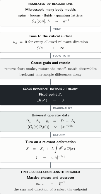
Different regulated systems can approach one fixed point after their relevant controls are tuned. Irrelevant differences decay toward the fixed-point operator data; turning on a relevant deformation then generates a finite correlation length and selects an infrared phase.

Universality Requires an Operator Dictionary

Suppose two microscopic models flow toward the same fixed point:

$$\mathcal S_A \longrightarrow \mathcal S_\star, \qquad \mathcal S_B \longrightarrow \mathcal S_\star.$$

This explains shared scaling dimensions and normalized scaling functions, but predictions still require maps

$$\begin{aligned} A_{\mathrm{lat}} &\longleftrightarrow \sum_i C_{A i}\mathcal O_i, \\ B_{\mathrm{lat}} &\longleftrightarrow \sum_i C_{B i}\mathcal O_i. \end{aligned}$$

The coefficients are generally nonuniversal. A fixed point without an operator dictionary does not tell an experimenter which probe measures which continuum correlation function.

What can be universal

With geometry and normalization specified, universal information can include:

• scaling dimensions and critical exponents;
• operator-product data;
• normalized scaling functions;
• selected amplitude ratios;
• fixed-point values of dimensionless observables;
• the number and symmetry of relevant directions.

What usually is not

The following are normally regulator or realization dependent:

• the critical temperature or microscopic coupling;
• the fixed-point coordinates in a chosen coupling chart;
• field-normalization constants;
• raw correlation and susceptibility amplitudes;
• the width of the observable scaling window;
• amplitudes of irrelevant corrections.

Universal data survive smooth changes of scheme. Bare and fixed-point coupling values generally do not.

Wilsonian Flow and Renormalized QFT

The Wilsonian and renormalized descriptions answer related questions with different bookkeeping.

Wilsonian convention

Let $k$ be a sliding infrared cutoff below a fixed ultraviolet cutoff $\Lambda$. Integrating modes above $k$ produces an action

$$\mathcal S_k[\phi].$$

With

$$\ell := \ln \frac{\Lambda}{k},$$

increasing $\ell$ means flowing toward the infrared. A coupling satisfies

$$\frac{d g_i}{d\ell} = \beta_i^{\mathrm{IR}}(\boldsymbol g).$$

Renormalization-scale convention

Perturbative QFT often uses a subtraction scale $\mu$ and defines

$$\beta_\mu(g) := \mu \frac{dg}{d\mu}.$$

If $\mu$ tracks $k$, then

$$\frac{dg}{d\ell} = -\beta_\mu(g).$$

A statement that a coupling “grows” is incomplete until the scale direction is declared.

Callan–Symanzik equation

For a critical renormalized $n$-point function in a one-coupling theory, one common convention is

$$\begin{aligned} 0 &= \Bigg[ \mu\frac{\partial}{\partial\mu} + \beta_\mu(g) \frac{\partial}{\partial g} \\ &\qquad+ n\gamma_\phi(g) \Bigg] G_R^{(n)}. \end{aligned}$$

Here

$$\gamma_\phi := \frac12 \mu \frac{d\ln Z_\phi}{d\mu}.$$

Masses, composite insertions, and several couplings add terms. At a fixed point,

$$\beta_\mu(g_\star) = 0,$$

and the anomalous dimension contributes to the scaling law. In this convention,

$$\eta = 2\gamma_\phi(g_\star).$$

The Callan–Symanzik equation expresses independence from the arbitrary subtraction scale after bare data are held fixed. It is not a physical-time evolution equation.

Counterterms and coarse graining are compatible

Counterterms define finite renormalized parameters and operators in a chosen scheme. Wilsonian integration explains why every allowed operator is generated and why long-distance predictions depend on only a few relevant coordinates near a fixed point. These are complementary formulations, not competing explanations.

Wilson–Fisher Fixed Point Preview

The $O(N)$ scalar model in

$$D = 4-\epsilon$$

dimensions gives the canonical perturbative bridge. Use the convention

$$\begin{aligned} \mathcal S &= \int d^D x\, \Bigg[ \frac12 (\partial_\mu\phi_a)^2 \\ &\qquad+ \frac12 r\phi_a^2 + \frac{ \mu^\epsilon g }{4!} (\phi_a\phi_a)^2 \Bigg]. \end{aligned}$$

The mass parameter must be tuned to its critical value $r_c(g)$. At $D=4$, $g$ is marginal by engineering power counting. For $D=4-\epsilon$, it is relevant at the Gaussian fixed point.

In minimal-subtraction-type conventions, the one-loop beta function is

$$\begin{aligned} \beta_\mu(g) &= -\epsilon g \\ &\quad+ \frac{N+8}{ 3(4\pi)^2 } g^2 + O(g^3). \end{aligned}$$

Besides the Gaussian fixed point, there is an interacting fixed point

$$g_\star = \frac{ 3(4\pi)^2 }{N+8} \epsilon + O(\epsilon^2).$$

Its coordinate depends on the normalization and scheme. The linearized slope

$$\beta_\mu'(g_\star) = \epsilon + O(\epsilon^2)$$

means that deviations in the quartic coupling decay as $\mu\to0$: this direction is infrared attractive.

The thermal eigenvalue and field anomalous dimension are

$$\begin{aligned} y_t &= 2 - \frac{N+2}{N+8} \epsilon + O(\epsilon^2), \\ \eta &= O(\epsilon^2). \end{aligned}$$

Therefore

$$\nu = \frac12 + \frac{N+2}{ 4(N+8) } \epsilon + O(\epsilon^2).$$

This small calculation displays the bridge:

1. a Landau–Ginzburg action supplies a regulated field theory;
2. loop renormalization supplies a beta function and anomalous dimensions;
3. a non-Gaussian fixed point replaces mean-field scaling;
4. stability eigenvalues become critical exponents;
5. the continuum QFT describes many microscopic realizations.

Setting $\epsilon=1$ at first order is only a rough estimate for three dimensions. Precision work needs higher orders, resummation, simulation, bootstrap, or other nonperturbative information. The displayed result is a preview of method, not a precision table.

Classical, Quantum, and Dynamic Criticality

The dimension entering a scaling relation must match the theory being scaled.

Thermal equilibrium criticality

For a static thermal transition in $d$ spatial dimensions, the long-distance statistical field theory is usually $D=d$ dimensional after massive temporal and microscopic modes have been integrated out.

Quantum criticality

At a zero-temperature quantum critical point,

$$\mathbf x \longmapsto b\mathbf x, \qquad \tau \longmapsto b^z\tau.$$

The integration measure scales with

$$D_{\mathrm{sc}} = d+z.$$

An eigenoperator can then obey

$$y_i = d+z-\Delta_i$$

when $\Delta_i$ is defined in this anisotropic convention. The notation $d+z$ is a scaling count, not a guarantee of an isotropic relativistic QFT.

Finite temperature gives an imaginary-time extent

$$L_\tau = \beta\hbar.$$

It stops the zero-temperature flow and creates the quantum-critical crossover regime developed on the dedicated quantum-transition page.

Dynamics is additional structure

The same static fixed point can support different dynamic universality classes. Conservation laws, damping, reversible couplings, noise, and hydrodynamic modes determine $z$ and real-time response. A static Euclidean functional does not choose those ingredients.

Hydrodynamics and Effective Theory Preview develops that real-time slow-variable and fluctuation framework; this page retains the static continuum and RG construction.

Scale Invariance Is Not Automatically Conformal

At an RG fixed point, the theory is scale invariant in the sense defined by the RG transformation. Conformal invariance is stronger.

Many familiar local, short-range, equilibrium critical points do admit a conformal description. When they do, conformal symmetry sharply constrains correlators and organizes operators into primaries and descendants.

One should not infer conformal symmetry from the words “fixed point” alone. The conclusion can depend on:

• locality and reflection positivity or unitarity;
• spacetime dimension;
• discreteness of the operator spectrum;
• conserved virial currents;
• anisotropic or nonrelativistic scaling;
• disorder and broad distributions;
• boundaries, defects, or long-range interactions.

Likewise, emergent rotational or Lorentz symmetry must be demonstrated by the flow of anisotropies and velocities. It is not guaranteed by taking a long wavelength limit.

Where the Simple Fixed-Point Picture Needs Extension

The ordinary isolated-fixed-point picture is powerful but not universal.

First-order transitions

A first-order transition has finite bulk correlation length except at a special endpoint. It does not generally define a scale-invariant continuum QFT by tuning to coexistence alone.

Berezinskii–Kosterlitz–Thouless transitions

Marginal flows and a fixed line produce an essential singularity rather than ordinary power-law tuning by one positive eigenvalue.

Fermi surfaces

Low-energy modes live near an extended momentum-space surface. Scaling is patch dependent, and four-fermion interactions require a channel-sensitive classification.

Disorder and infinite-randomness flow

The running object can be a probability distribution rather than a finite set of couplings. Typical and average observables can scale differently.

Boundaries and defects

A bulk fixed point can coexist with independent boundary or defect operators, relevant perturbations, and universality classes.

Several soft sectors

Order parameters coupled to gauge fields, Goldstone modes, fermions, or hydrodynamic densities can generate nonlocal kernels and additional relevant directions. Integrating out a gapless field does not generally leave a local polynomial action.

Exact and Approximate Statements

Keep the following statuses separate.

• Exact at fixed regulator: change variables with the Jacobian, integrate a declared shell, differentiate a convergent generating functional, or preserve the partition function under a normalized block map.
• Definition dependent: choose the field normalization, cutoff, coupling chart, subtraction scheme, or operator basis.
• Linearized statement: classify eigen-directions using the stability matrix sufficiently near a fixed point.
• Perturbative approximation: truncate a loop or $\epsilon$ expansion.
• Effective-field-theory truncation: retain a finite operator set and estimate the omitted terms.
• Continuum-limit claim: show regulator-independent predictions along a tuned trajectory.
• Universality claim: match several asymptotic observables and exclude plausible competing classes.
• Conformal claim: establish the extra assumptions and tests beyond scale invariance.

An exact coarse-graining identity can be followed by an uncontrolled truncation. A low-order approximation can also be quantitatively useful when its expansion parameter and uncertainty are explicit.

A Reliable Bridge Workflow

1. Establish a continuous transition

Distinguish continuous, first-order, crossover, and essential-singularity behavior before invoking an isolated critical fixed point.

2. Declare the regulator

Specify lattice spacing or cutoff, volume, boundaries, fields, and measure.

3. Identify every soft mode

Include the order parameter, conserved densities, gauge fields, defects, fermions, and other gapless sectors relevant to the scale window.

4. Match microscopic observables

Give their symmetry, normalization, sources, and expansion in continuum operators.

5. Write the allowed continuum action

Include every operator allowed by the retained symmetries to the stated order.

6. Fix the flow convention

State whether the independent scale increases toward the infrared or toward the ultraviolet.

7. Find and test candidate fixed points

Do not infer the endpoint solely from a runaway truncation or one perturbative zero.

8. Count physical relevant directions

Remove directions forbidden by exact symmetry and identify redundant coordinates before counting experimental tuning controls.

9. Compute operator data

Use beta functions, anomalous-dimension matrices, simulations, exact methods, or nonperturbative tools with their uncertainties.

10. Control the scaling window

Track $a$, $\xi$, $L$, temperature, frequency, and irrelevant correction scales.

11. Compare several observables

Test exponents, normalized correlators, dimensionless ratios, and operator selection rules rather than one fitted power.

12. State the continuation

Separate the many-body interpretation from the full QFT tasks of loop renormalization, composite-operator mixing, Ward identities, and nonperturbative continuum construction.

Common Mistakes

• Calling any long-wavelength approximation a continuum limit without showing $\xi/a\to\infty$.
• Sending $a\to0$ while holding every bare coupling fixed.
• Identifying a lattice observable with one continuum field without operator matching.
• Treating a critical fixed point as necessarily Gaussian.
• Reading the numerical fixed-point coupling as universal.
• Classifying bare monomials before resolving operator mixing.
• Saying “relevant” without naming the fixed point and scale direction.
• Confusing a renormalization scale with physical time.
• Treating counterterms as unrelated to Wilsonian effective actions.
• Assuming one vanishing mass parameter tunes every relevant deformation.
• Equating $d+z$ with a literal isotropic dimension.
• Inferring Lorentz or conformal invariance from scale invariance alone.
• Using a static universality class to predict dynamics.
• Taking first-order $\epsilon=1$ estimates as precision three-dimensional results.
• Dropping irrelevant operators before checking corrections or dangerous irrelevance.
• Claiming universality from one exponent or a visually pleasing collapse.
• Removing the regulator before renormalized observables and matching conditions are defined.

Connections

• Statistical Field Theory Preview supplies the regulated measure whose long-distance flow is analyzed here.
• Renormalization Group Preview develops the Wilsonian transformation and flow geometry in depth.
• Critical Exponents and Scaling turns the eigenvalues introduced here into thermodynamic, correlation, and finite-size predictions.
• Universality gives the full classification and evidence standard.
• Landau–Ginzburg Theory Preview supplies the scalar functional used in the Wilson–Fisher example.
• Quantum Phase Transitions develops anisotropic scaling and quantum-critical crossover.
• Finite-Temperature QFT Bridge develops the compact thermal direction, Matsubara scales, screening, and the conditions for a static lower-dimensional effective theory.
• Connected Correlation Functions owns clustering, connected subtraction, and correlation-length definitions.
• Sources to Generating Functionals develops source differentiation and connected functionals.
• Continue on QFT.org tracks the planned renormalization, RG, and EFT destination and the current live fallback without presenting an unpublished route as available.

References

1. L. P. Kadanoff, “Scaling Laws for Ising Models near $T_c$”, Physics Physique Fizika 2, 263–272 (1966) – block variables and scaling.
2. K. G. Wilson, “Renormalization Group and Critical Phenomena. I. Renormalization Group and the Kadanoff Scaling Picture”, Physical Review B 4, 3174–3183 (1971) – fixed points and the Kadanoff picture.
3. K. G. Wilson, “Renormalization Group and Critical Phenomena. II. Phase-Space Cell Analysis of Critical Behavior”, Physical Review B 4, 3184–3205 (1971) – critical behavior from repeated coarse graining.
4. F. J. Wegner, “Corrections to Scaling Laws”, Physical Review B 5, 4529–4536 (1972) – nonlinear scaling fields and irrelevant corrections.
5. K. G. Wilson and M. E. Fisher, “Critical Exponents in 3.99 Dimensions”, Physical Review Letters 28, 240–243 (1972) – the original $\epsilon$-expansion fixed point.
6. K. G. Wilson and J. Kogut, “The Renormalization Group and the $\epsilon$ Expansion”, Physics Reports 12, 75–200 (1974) – the statistical-field and QFT synthesis.
7. M. E. Fisher, “The Renormalization Group in the Theory of Critical Behavior”, Reviews of Modern Physics 46, 597–616 (1974) – scaling fields and universal critical behavior.
8. C. G. Callan, Jr., “Broken Scale Invariance in Scalar Field Theory”, Physical Review D 2, 1541–1547 (1970) – renormalization-scale equations for field-theory amplitudes.
9. J. Polchinski, “Renormalization and Effective Lagrangians”, Nuclear Physics B 231, 269–295 (1984) – Wilsonian flow and perturbative renormalizability.
10. J. A. Hertz, “Quantum Critical Phenomena”, Physical Review B 14, 1165–1184 (1976) – field theory for quantum critical systems.
11. P. C. Hohenberg and B. I. Halperin, “Theory of Dynamic Critical Phenomena”, Reviews of Modern Physics 49, 435–479 (1977) – the distinction between static and dynamic universality.
12. A. Pelissetto and E. Vicari, “Critical Phenomena and Renormalization-Group Theory”, Physics Reports 368, 549–727 (2002) – high-precision critical field theory and universality.
13. J. Cardy, Scaling and Renormalization in Statistical Physics, Cambridge University Press (1996) – scaling operators, universality, and continuum limits.
14. S. Sachdev, Quantum Phase Transitions, 2nd ed., Cambridge University Press (2011) – quantum critical scaling and continuum field theories.
15. M. E. Fisher, “Renormalization Group Theory: Its Basis and Formulation in Statistical Physics”, Reviews of Modern Physics 70, 653–681 (1998) – conceptual foundations and statistical applications.

Exercises

1. Tune a Massive Continuum Limit

Suppose a lattice correlation length obeys

$$\xi_{\mathrm{lat}}(t) = A \lvert t\rvert^{-\nu},$$

where $\xi_{\mathrm{lat}}$ is measured in lattice spacings. Find how $t$ must depend on $a$ so that the physical correlation length $\xi_{\mathrm{phys}}=a\xi_{\mathrm{lat}}$ approaches a fixed nonzero value $\Xi$ as $a\to0$.

Solution

Require

$$\Xi = aA \lvert t(a)\rvert^{-\nu}.$$

Solving gives

$$\lvert t(a)\rvert = \left( \frac{Aa}{\Xi} \right)^{1/\nu}.$$

Thus $t(a)\to0$ as the cutoff is removed. Meanwhile,

$$\frac{\xi_{\mathrm{phys}}}{a} = \frac{\Xi}{a} \longrightarrow \infty.$$

The continuum theory is massive because $m_{\mathrm{corr}}=\Xi^{-1}$ remains finite, but its bare lattice control is tuned toward the critical point.

2. Operators and Coupling Eigenvalues

In an isotropic $D=3$ fixed-point theory, four scalar eigenoperators have dimensions

$$\Delta \in \{1.04,\ 2.40,\ 3.00,\ 4.20\}.$$

Classify their integrated couplings at linear order and give each RG eigenvalue.

Solution

For an integrated scalar deformation,

$$y = D-\Delta = 3-\Delta.$$

Therefore:

$$\begin{aligned} \Delta=1.04,\quad y=1.96 &: \text{relevant}, \\ \Delta=2.40,\quad y=0.60 &: \text{relevant}, \\ \Delta=3.00,\quad y=0 &: \text{marginal}, \\ \Delta=4.20,\quad y=-1.20 &: \text{irrelevant}. \end{aligned}$$

The $\Delta=3$ operator requires the nonlinear beta function. Symmetry can forbid a relevant operator, and redundant operators must be removed before counting physical tuning directions.

3. Correlation Length as an RG Stopping Scale

Let one relevant field obey

$$u(b) = b^y u, \qquad y>0.$$

Derive the correlation-length exponent and the corresponding mass scaling.

Solution

The flow leaves the fixed-point neighborhood when

$$b_\star^y \lvert u\rvert \sim 1.$$

Hence

$$b_\star \sim \lvert u\rvert^{-1/y}.$$

The only generated long length is

$$\xi \sim a b_\star \sim a \lvert u\rvert^{-1/y}.$$

Comparing with $\xi\sim\lvert u\rvert^{-\nu}$ gives

$$\nu = \frac{1}{y}.$$

The inverse-correlation-length mass behaves as

$$m_{\mathrm{corr}}a \sim \frac{a}{\xi} \sim \lvert u\rvert^{1/y} = \lvert u\rvert^\nu.$$

4. Leading Operator in a Lattice Correlator

A $\mathbb Z_2$-odd lattice observable has the continuum expansion

$$A_{\mathrm{lat}} = c_1\sigma + c_2\mathcal O_{\mathrm{odd}} + \cdots,$$

with

$$\Delta_\sigma < \Delta_{\mathrm{odd}}.$$

What controls the leading long-distance two-point function? What changes if $c_1=0$?

Solution

When $c_1\ne0$, the smallest-dimension allowed operator dominates:

$$\begin{aligned} \left\langle A_{\mathrm{lat}}(x) A_{\mathrm{lat}}(0) \right\rangle_{\mathrm c} &\sim c_1^2 \\ &\quad\times \frac{C_\sigma}{ \lvert x\rvert^{2\Delta_\sigma} }. \end{aligned}$$

The amplitude $c_1^2C_\sigma$ depends on microscopic normalization, while the power is fixed by the continuum operator dimension.

If symmetry, an improved-observable construction, or an accidental cancellation gives $c_1=0$, then the next operator with nonzero coefficient controls the asymptotic power:

$$\lvert x\rvert^{-2\Delta_{\mathrm{odd}}}.$$

This is why an operator dictionary needs overlap coefficients as well as a list of allowed symmetries.

5. One-Loop Wilson–Fisher Data

Use

$$\beta_\mu(g) = -\epsilon g + A_N g^2, \qquad A_N = \frac{N+8}{ 3(4\pi)^2 }.$$

Find the interacting fixed point and its slope. Then use the first-order formula for $\nu$ to estimate the $N=1$, $D=3$ value.

Solution

The nonzero root is

$$g_\star = \frac{\epsilon}{A_N} = \frac{ 3(4\pi)^2 }{N+8} \epsilon.$$

The slope is

$$\begin{aligned} \beta_\mu'(g_\star) &= -\epsilon + 2A_Ng_\star \\ &= \epsilon. \end{aligned}$$

Thus a small deviation obeys

$$\delta g(\mu) \propto \mu^\epsilon$$

and decays toward the infrared when $\epsilon>0$.

For $N=1$ and $\epsilon=1$,

$$\begin{aligned} \nu &\simeq \frac12 + \frac{3}{36} \\ &= \frac{7}{12} \simeq 0.583. \end{aligned}$$

This is a first-order estimate, not the precision three-dimensional Ising value. The discrepancy measures the need for higher orders and controlled resummation or nonperturbative methods.

6. Translate the Beta-Function Sign

Let

$$\ell = \ln \frac{\Lambda}{\mu}.$$

Show how a QFT beta function

$$\beta_\mu(g) = \mu\frac{dg}{d\mu}$$

is related to the infrared-length convention

$$\beta_{\mathrm{IR}}(g) := \frac{dg}{d\ell}.$$

Solution

Because

$$\frac{d\ell}{d\ln\mu} = -1,$$

the chain rule gives

$$\begin{aligned} \beta_{\mathrm{IR}}(g) &= \frac{dg}{d\ell} \\ &= -\frac{dg}{d\ln\mu} \\ &= -\beta_\mu(g). \end{aligned}$$

The zeros are the same, but arrows on a flow diagram reverse. Relevance and stability statements must therefore name the convention.

7. Count the Required Tunings

A candidate fixed point has three relevant eigenoperators:

• an even thermal operator $\varepsilon$;
• an odd magnetic operator $\sigma$;
• an even anisotropy operator $\mathcal A$.

How many controls must be tuned with and without exact $\mathbb Z_2$ symmetry?

Solution

Without an exact symmetry, all three relevant couplings are allowed. Reaching the fixed point generically requires tuning three independent controls.

Exact $\mathbb Z_2$ symmetry forbids the odd source coupled to $\sigma$, so that coordinate is fixed to zero by symmetry. The even thermal and anisotropy couplings remain allowed and relevant. Two controls must still be tuned.

Symmetry reduces the accessible coupling space; it does not make every remaining relevant operator vanish.

8. Susceptibility from a Fixed-Point Correlator

At criticality in $D$ dimensions, suppose

$$\left\langle \phi(x)\phi(0) \right\rangle_{\mathrm c} \sim \frac{1}{ \lvert x\rvert^{D-2+\eta} }.$$

Estimate the finite-size scaling of the zero-momentum susceptibility in a box of linear size $L$.

Solution

Ignoring geometry-dependent constants and the ultraviolet contact region,

$$\begin{aligned} \chi_L &\sim \int_a^L dr\, r^{D-1} r^{-(D-2+\eta)} \\ &= \int_a^L dr\, r^{1-\eta}. \end{aligned}$$

For $2-\eta>0$, the upper limit dominates:

$$\chi_L \sim L^{2-\eta}.$$

The cutoff-dependent lower-limit contribution is analytic background. The leading infrared power is fixed by the continuum scaling dimension

$$2\Delta_\phi = D-2+\eta.$$