Critical Exponents and Scaling

Critical exponents describe how observables become singular near a continuous critical point; scaling theory explains why those exponents, scaling functions, and finite-size trends are linked rather than independent fit parameters.

The broader Finite-Size Effects page diagnoses physical size mechanisms before critical scaling is assumed. This page owns the special asymptotic theory once a continuous critical regime and its scaling fields are the working hypothesis.

If $u$ measures distance from criticality, a leading power law has the form

$$O_{\mathrm{sing}}(u) \sim A_\pm \lvert u\rvert^{\kappa}.$$

The exponent $\kappa$ describes the asymptotic power. The amplitudes $A_+$ and $A_-$ can differ on the two sides of the transition. Neither the power law nor its fitted exponent is meaningful until the control variable, limiting path, observable normalization, regular background, and scaling window are stated.

Scaling theory is stronger than a list of powers. It asserts that the singular dependence on several controls can be organized by homogeneous functions. Consequences include:

• relations among bulk exponents;
• universal limiting shapes after nonuniversal metric factors are fixed;
• finite-size rounding and pseudocritical drift;
• dynamic scaling through a time-length exponent;
• systematic corrections from irrelevant fields, boundaries, and analytic backgrounds;
• quantitative consistency tests across observables.

Canonical Scope

This page is the canonical home for:

• the static exponent dictionary $\alpha$, $\beta_{\mathrm{op}}$, $\gamma$, $\delta$, $\nu$, and $\eta$;
• the dynamic critical exponent $z$;
• homogeneous scaling of the singular free energy;
• Widom, Rushbrooke, Fisher, and hyperscaling relations, with their assumptions;
• finite-size scaling of order parameters, susceptibilities, gaps, and dimensionless ratios;
• pseudocritical shifts, crossing drift, and corrections to scaling;
• scaling-collapse construction and statistical validation;
• upper-critical-dimension, dangerous-irrelevance, logarithmic, anisotropic, and essential-scaling caveats;
• mean-field and two-dimensional Ising benchmarks;
• the thermal-to-quantum scaling dictionary.

Neighboring pages retain separate ownership:

• Finite-Temperature Phase Transitions defines thermal transition order, coexistence, critical temperature, and finite-size rounding.
• Quantum Phase Transitions defines zero-temperature critical points, quantum-critical fans, and benchmark Hamiltonians.
• Order Parameters owns operator, source, component, and normalization choices.
• Connected Correlation Functions owns connected subtraction, clustering, and correlation-length definitions.
• Susceptibilities owns static and dynamic response conventions.
• Thermodynamic Limit owns limiting sequences, boundary conditions, and noncommuting limits.
• Mean-Field Theory owns self-consistent approximations and their control criteria.
• Landau Theory owns the uniform analytic potential, its minimization, and the derivation of mean-field thermodynamic exponents.

Universality owns universality-class classification. Renormalization Group Preview owns coarse-graining flow in depth. Critical Phenomena and RG Bridge translates scaling fields and operator dimensions into continuum-QFT language. This page uses only the scaling-field language needed to state and test critical behavior. The Critical Exponent Glossary is the compact lookup companion for definitions, assumptions, and notation collisions.

Controls, Sources, and Scaling Fields

Thermal control

For a transition at $T_c\gt0$, define the reduced temperature

$$t := \frac{T-T_c}{T_c}.$$

Then $t\to0^+$ approaches from above and $t\to0^-$ from below. Some communities reverse this sign. A reported amplitude ratio is meaningless unless that convention is explicit.

Quantum control

For a zero-temperature transition driven by a coupling $g$,

$$\delta := \frac{g-g_c}{g_0},$$

where $g_0$ is a fixed microscopic scale. If $g$ is already dimensionless, one may take $g_0=1$.

Ordering source

For an intensive order parameter $m$ and conjugate source $h$,

$$H(h) := H(0)-hM, \qquad m := \frac{\langle M\rangle}{V}.$$

The source direction can matter for vector or tensor order. The limits $h\to0$ and $V\to\infty$ must also be ordered when spontaneous symmetry breaking is possible.

Physical controls are not always scaling fields

The variables that transform simply near the critical point are analytic scaling fields. For example,

$$\begin{aligned} u_t &= a_t t + a_{tt}t^2 + a_{th}h^2 + \cdots, \\ u_h &= a_h h + a_{ht}ht + \cdots. \end{aligned}$$

Symmetry constrains the allowed mixing. In an Ising-symmetric problem, $u_t$ is even and $u_h$ is odd under $h\mapsto-h$. In a fluid, the experimentally controlled temperature and chemical potential can mix into both thermal and ordering fields.

Close enough to criticality, $u_t\propto t$ and $u_h\propto h$. Outside that asymptotic region, nonlinear field mixing can imitate a changed exponent or skew a collapse.

Singular and Regular Parts

Write a thermodynamic potential density as

$$f(t,h) = f_{\mathrm{reg}}(t,h) + f_{\mathrm s}(t,h).$$

The regular part is analytic near the critical point. The singular part carries the nonanalytic long-distance contribution.

This decomposition matters because measurements and simulations see their sum. For example,

$$c_h(t) = c_{\mathrm{reg}}(t) + c_{\mathrm s}(t).$$

If $\alpha<0$, the singular heat-capacity contribution vanishes at criticality while a cusp remains in a derivative. A smooth background can then dominate the raw signal. If $\alpha=0$, the leading singularity can be logarithmic rather than a nonzero constant power.

Additive backgrounds cannot generally be removed by multiplying the data by a power of $L$. They must be modeled, subtracted with justified uncertainty, or avoided by choosing a cleaner observable.

The Static Exponent Dictionary

The standard symbols refer to specified asymptotic paths. They are not labels for arbitrary slopes on log-log plots.

Correlation-length exponent

At zero source,

$$\xi_\pm(t) \sim \xi_\pm^{(0)} \lvert t\rvert^{-\nu}.$$

The exponent $\nu$ controls the diverging length scale. The amplitudes $\xi_+^{(0)}$ and $\xi_-^{(0)}$ are generally different.

Order-parameter exponent

On the ordered side at zero source,

$$m(t,0) \sim B(-t)^{\beta_{\mathrm{op}}}, \qquad t\to0^-.$$

The subscript on $\beta_{\mathrm{op}}$ distinguishes this exponent from inverse temperature.

Susceptibility exponent

For the response conjugate to $h$,

$$\chi(t,0) \sim \Gamma_\pm \lvert t\rvert^{-\gamma}.$$

One must keep fixed the ensemble and source normalization that define $\chi$.

Critical-isotherm exponent

At $t=0$,

$$m(0,h) \sim D\, \operatorname{sgn}(h) \lvert h\rvert^{1/\delta}.$$

This $\delta$ is an exponent, not the reduced quantum control used elsewhere on this page.

Heat-capacity exponent

The singular heat capacity at zero source is conventionally written

$$c_{\mathrm s}(t) \sim A_\pm \lvert t\rvert^{-\alpha}.$$

Special care is required at $\alpha=0$. The two-dimensional Ising model, for example, has

$$c_{\mathrm s}(t) \sim -A\ln\lvert t\rvert,$$

not an ordinary finite jump.

Anomalous-dimension exponent

At criticality, the connected order-parameter correlation function commonly obeys

$$G_c(r) \sim \frac{A_G}{ r^{d-2+\eta} }.$$

The exponent $\eta$ measures the departure from the Gaussian power $d-2$. Landau–Ginzburg Theory Preview derives the Gaussian benchmarks $\eta=0$ and $\nu=1/2$ from the spatial quadratic kernel. The formula here assumes isotropic short-range scaling and distances large compared with the microscopic cutoff.

Dynamic exponent

When one critical time scale is tied to the correlation length,

$$\tau_{\mathrm{rel}} \sim \xi^z.$$

Equivalently, a characteristic frequency or gap scales as

$$\omega_\xi \sim \xi^{-z}.$$

Static exponents do not determine $z$. At a thermal transition, conservation laws and the chosen dynamics can change $z$ without changing the equilibrium static exponents. At a quantum critical point, $z$ also controls the scaling of imaginary time relative to space.

Homogeneous Scaling of the Free Energy

For an isotropic thermal critical point, a standard scaling hypothesis is

$$\begin{gathered} f_{\mathrm s} \left( u_t,u_h,\{u_i\} \right) = b^{-d} \\ {}\times \mathcal F_f \left( X_t,X_h,\{X_i\} \right), \\ X_t := u_t b^{y_t}, \qquad X_h := u_h b^{y_h}, \\ X_i := u_i b^{y_i}. \end{gathered}$$

Here:

• $b\gt1$ is a change of length scale;
• $y_t\gt0$ and $y_h\gt0$ are relevant scaling eigenvalues;
• $u_i$ are additional scaling fields;
• $y_i<0$ denotes an irrelevant field;
• $y_i=0$ denotes a marginal field requiring separate analysis.

The thermal eigenvalue defines

$$y_t := \frac{1}{\nu}.$$

Choosing

$$b = \lvert u_t\rvert^{-\nu}$$

gives

$$f_{\mathrm s}(t,h) \sim \lvert t\rvert^{d\nu} \mathcal F_\pm \left( \frac{h}{ \lvert t\rvert^{\nu y_h} } \right),$$

up to nonuniversal metric factors and irrelevant-field corrections.

The prefactor $b^{-d}$ is the hyperscaling assumption that one correlated volume contributes an order-one singular free energy. It is powerful, but it is not universally valid.

Deriving the Exponent Relations

The order parameter is a source derivative:

$$m = -\frac{\partial f_{\mathrm s}}{\partial h}.$$

Its scaling dimension is therefore $d-y_h$, giving

$$\beta_{\mathrm{op}} = \nu \left( d-y_h \right).$$

A second source derivative gives

$$\gamma = \nu \left( 2y_h-d \right).$$

At $t=0$, choose $b=\lvert h\rvert^{-1/y_h}$. Then

$$\delta = \frac{y_h}{ d-y_h }.$$

The critical correlator fixes the source eigenvalue:

$$y_h = \frac{ d+2-\eta }{2}.$$

Finally, differentiating the singular free energy twice with respect to temperature gives, when hyperscaling holds,

$$2-\alpha = d\nu.$$

Combining these equations yields the familiar relations

$$\begin{aligned} \alpha + 2\beta_{\mathrm{op}} + \gamma &= 2, \\ \gamma &= \beta_{\mathrm{op}} \left( \delta-1 \right), \\ \gamma &= \nu \left( 2-\eta \right), \\ 2-\alpha &= d\nu. \end{aligned}$$

These are commonly called the Rushbrooke, Widom, Fisher, and hyperscaling relations. The first three follow from a conventional two-field scaling form; the last also uses the correlation-volume hypothesis.

They are conditional identities, not definitions. Long-range interactions, multiple length scales, dangerous irrelevant variables, quenched disorder, constraints, or non-power-law criticality can require modified relations. Earlier rigorous thermodynamic arguments often establish inequalities under weaker assumptions; equality needs the scaling hypothesis.

Scaling Equation of State

The same homogeneity relation organizes the full critical equation of state:

$$m(t,h) = \lvert t\rvert^{\beta_{\mathrm{op}}} \mathcal M_\pm \left( \frac{h}{ \lvert t\rvert^{\beta_{\mathrm{op}}\delta} } \right).$$

An equivalent form is

$$h = \lvert m\rvert^\delta \operatorname{sgn}(m) \mathcal H \left( \frac{t}{ \lvert m\rvert^{1/\beta_{\mathrm{op}}} } \right).$$

These expressions connect the coexistence curve, susceptibility, and critical isotherm. They also show why fitting $m(t,0)$, $\chi(t,0)$, and $m(0,h)$ independently wastes information: all three are limits of one scaling function.

The scaling functions are not universal until conventions are fixed. Rescaling $t$, $h$, and $m$ changes their metric factors. Properly normalized shapes and selected amplitude ratios can be universal within a universality class and fixed geometry.

Correlations, Structure Factors, and Susceptibility

Away from criticality, a common scaling form is

$$G_c(r,t) = \frac{1}{ r^{d-2+\eta} } \mathcal G_\pm \left( \frac{r}{\xi} \right).$$

Fourier transformation gives the static structure factor

$$S_c(q,t) = \xi^{2-\eta} \mathcal S_\pm(q\xi),$$

up to normalization and contact terms.

At zero momentum,

$$\chi \propto S_c(0,t) \sim \xi^{2-\eta},$$

which reproduces

$$\gamma = \nu(2-\eta).$$

The proportionality between a fluctuation and a susceptibility depends on temperature factors, source conventions, ensemble constraints, and whether the relevant operators commute. Fluctuations and Susceptibilities develops those exact identities.

Dynamic Scaling

With one critical length and one critical time, a retarded susceptibility can be organized schematically as

$$\chi^R(q,\omega;t) = \xi^{2-\eta} \mathcal X_\pm \left( q\xi, \omega\xi^z \right).$$

The exact prefactor and scaling function depend on the operator and response convention. The dimensionless variables $q\xi$ and $\omega\xi^z$ express the robust content.

Critical slowing down follows from

$$\tau_{\mathrm{rel}} \sim \lvert t\rvert^{-\nu z}.$$

For classical stochastic dynamics, two systems with the same static Hamiltonian can have different $z$ if one conserves the order parameter and the other does not. Hydrodynamic couplings can introduce additional slow modes.

For a quantum critical point,

$$\Delta \sim \xi^{-z} \sim \lvert\delta\rvert^{\nu z},$$

where $\Delta$ is the appropriate bulk excitation scale. A collapsing symmetry-partner splitting inside an ordered phase is not automatically this critical gap.

Finite-Size Scaling

A finite sample cannot realize $\xi=\infty$. Once $\xi$ reaches the system size, $L$ becomes the infrared cutoff.

For an observable of scaling dimension $x_O$,

$$\begin{aligned} O_L(t) ={}& L^{-x_O} \left[ \Phi_O \left( tL^{1/\nu} \right) \right. \\ & \left. + L^{-\omega} \Phi_{O,1} \left( tL^{1/\nu} \right) + \cdots \right], \end{aligned}$$

where $\omega\gt0$ is the leading correction-to-scaling exponent. Analytic backgrounds may need to be added separately.

Common specializations are

$$\begin{aligned} m_L(t) &= L^{-\beta_{\mathrm{op}}/\nu} \mathcal M_L(x), \\ \chi_L(t) &= L^{\gamma/\nu} \mathcal X_L(x), \\ \frac{\xi_L(t)}{L} &= \mathcal R_\xi(x), \\ U_{4,L}(t) &= \mathcal R_U(x), \\ x &:= tL^{1/\nu}. \end{aligned}$$

The Binder ratio $U_{4,L}$ depends on its component and normalization convention. The ratio $\xi_L/L$ depends on how the finite-size correlation length is defined.

Peak locations, widths, and heights

If a response scaling function has a maximum at $x=x^\star$, then

$$t_L^\star \sim x^\star L^{-1/\nu}.$$

Its width scales as

$$\delta t_L \sim L^{-1/\nu},$$

and a susceptibility peak scales as

$$\chi_L^{\max} \sim L^{\gamma/\nu}.$$

These leading powers can be obscured by backgrounds, corrections, boundary terms, or a peak whose location lies outside the asymptotic scaling window.

Dimensionless crossings and drift

For a dimensionless ratio $R_L$ near criticality, write

$$R_L(t) = R^\star + a\,tL^{1/\nu} + b\,L^{-\omega} + \cdots.$$

For a fixed size ratio $s\gt1$, the crossing of sizes $L$ and $sL$ then drifts as

$$t_\times(L,sL) \simeq \frac{ b(1-s^{-\omega}) }{ a(s^{1/\nu}-1) } L^{-(1/\nu+\omega)}.$$

A crossing that visibly moves is not defective data. It is expected when irrelevant fields are appreciable. Ignoring that drift can bias both $T_c$ and $\nu$.

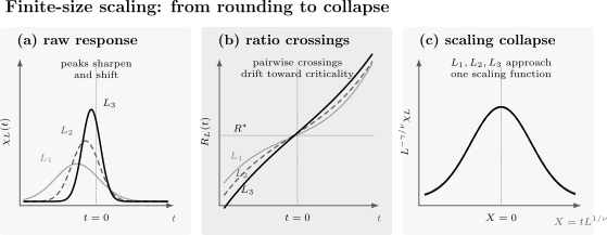
Three stages of finite-size reasoning. Raw response curves sharpen and shift with $L$. A dimensionless ratio approaches a common critical value but its pairwise crossings can drift because of corrections. Under the correct asymptotic hypothesis, plotting $L^{x_O}O_L$ against $x=tL^{1/\nu}$ removes the leading size dependence over a stated scaling window.

Geometry and boundary conditions

Finite-size scaling functions depend on:

• boundary conditions;
• aspect ratio;
• sample shape;
• anisotropy;
• the observable’s position relative to a boundary;
• whether spatial and imaginary-time extents are scaled together.

Critical exponents can remain unchanged while the crossing value $R^\star$ changes. Comparing Binder ratios from different geometries without conversion is therefore unsafe.

Scaling Collapse

Suppose

$$O_L(t) = L^{-x_O} \Phi_O \left( tL^{1/\nu} \right).$$

Define rescaled coordinates

$$X := tL^{1/\nu}, \qquad Y := L^{x_O}O_L.$$

If the leading scaling hypothesis applies, data from different sizes approach one curve $Y=\Phi_O(X)$.

What a collapse tests

A successful collapse tests compatibility among:

• the candidate critical point;
• the exponent $\nu$;
• the observable dimension $x_O$;
• the chosen scaling window;
• the neglect or inclusion of correction terms.

It does not independently prove all of them. With enough adjustable parameters and a narrow plotting range, visually persuasive but incorrect collapses are easy to produce.

A defensible collapse workflow

1. Define the observable, source, ensemble, boundaries, and size variable.
2. Estimate autocorrelation times and construct statistically meaningful bins.
3. Locate a plausible critical region using dimensionless crossings or independent diagnostics.
4. Specify a minimum size $L_{\min}$ and a maximum rescaled distance $\lvert X\rvert_{\max}$.
5. Fit the raw data to a scaling model, including corrections when supported.
6. Propagate uncertainty in $T_c$, exponents, nuisance parameters, and the scaling function.
7. Repeat over several $L_{\min}$ and window choices.
8. Test another observable with the same critical point and compatible exponents.
9. Compare against first-order, crossover, logarithmic, or essential-scaling alternatives.
10. Plot the collapse only after reporting the inference procedure.

Correlated data

Values obtained from histogram reweighting, shared disorder samples, common normalization, or repeated processing of one Monte Carlo chain are correlated.

For a residual vector $\mathbf r$ with covariance matrix $C$, the Gaussian quadratic form is

$$\chi_C^2 := \mathbf r^{\mathsf T} C^{-1} \mathbf r.$$

Replacing $C$ by only its diagonal generally overcounts information. If $C$ is poorly conditioned, one should use justified regularization, coarser independent summaries, or a resampling procedure that preserves the correlation structure.

Bootstrap or jackknife resampling should act on independent simulation bins or disorder realizations, not on already correlated plotted points. The entire fitting pipeline, including critical-point location and scaling-function estimation, should be repeated inside each resample.

The unknown scaling function

The function $\Phi_O$ is usually not known. Common representations include:

• a low-order polynomial over a narrow $X$ window;
• splines with controlled smoothness;
• orthogonal basis expansions;
• Gaussian-process or other regularized nonparametric models.

The representation must be flexible enough not to force the answer and constrained enough not to interpolate noise. Model complexity, fit range, and priors are part of the reported analysis.

Corrections to Scaling

Irrelevant fields

If the leading irrelevant field has eigenvalue

$$y_u = -\omega, \qquad \omega\gt0,$$

then it produces corrections proportional to $L^{-\omega}$ at criticality or $\lvert t\rvert^{\nu\omega}$ in the bulk.

The amplitude of that correction is nonuniversal. It can accidentally be small, change sign, or be tuned close to zero in an improved model.

Nonlinear scaling fields

Because

$$u_t = a_t t + a_{tt}t^2 + \cdots,$$

the true scaling coordinate is

$$u_t L^{1/\nu},$$

not necessarily $tL^{1/\nu}$ outside the narrow asymptotic region.

Analytic backgrounds

An observable may have

$$O_L(t) = O_{\mathrm{reg}}(t) + O_{\mathrm s,L}(t).$$

The regular term can dominate when the singular exponent is small or negative. Derivatives, ratios, or explicitly background-aware fits may be more stable than naive multiplication by a power of $L$.

Boundary and shape corrections

Open boundaries add surface, edge, and corner contributions. Their powers need not equal $\omega$. Aspect-ratio drift can also masquerade as a bulk correction.

Competing correction exponents

If several corrections are comparable, a one-power fit can return an effective exponent with no asymptotic meaning. The remedy is not automatically to add many unconstrained powers. One needs larger sizes, improved observables, independent theory input, or an honest statement that the asymptotic regime has not been reached.

Auxiliary Exponents and Stability Checks

The RG eigenvalues provide a compact dictionary for the primary exponents. For ordinary isotropic scaling,

$$y_t=\frac1\nu, \qquad y_h=\frac{d+2-\eta}{2}, \qquad y_i=-\omega<0,$$

where $y_t$ and $y_h$ are the relevant thermal and ordering-field eigenvalues and $\omega$ is the leading correction-to-scaling exponent. If a second relevant field $g$ has eigenvalue $y_g$, a commonly used crossover variable is $g\lvert t\rvert^{-\phi}$ with $\phi=y_g/y_t$; authors must state the convention because $\phi$ is not universal notation.

Quenched short-range disorder is perturbatively irrelevant at a clean classical critical point when the Harris condition $d\nu>2$ holds. If disorder produces a conventional random fixed point, the Chayes bound gives $\nu\ge 2/d$ under its stated assumptions. These are diagnostic constraints, not substitutes for identifying the fixed point: correlated disorder, anisotropic scaling, activated dynamics, or unconventional finite-size lengths require a separate analysis.

Upper Critical Dimensions and Dangerous Irrelevance

For a short-range scalar $\phi^4$ theory, the static upper critical dimension is

$$d_c = 4.$$

Below $d_c$, fluctuations change the mean-field powers and ordinary hyperscaling can hold. At $d=d_c$, marginality commonly produces logarithmic corrections. Above $d_c$, bulk exponents take mean-field values, but ordinary hyperscaling fails.

The mean-field values

$$\begin{aligned} \alpha&=0, & \beta_{\mathrm{op}}&=\frac12, & \gamma&=1, \\ \delta&=3, & \nu&=\frac12, & \eta&=0 \end{aligned}$$

give

$$2-\alpha = 2,$$

whereas

$$d\nu = \frac d2.$$

The two agree only at $d=4$.

The quartic coupling is irrelevant at the Gaussian fixed point above $d_c$, yet setting it to zero destroys the stable ordered phase and changes some singular limits. It is therefore dangerously irrelevant. Standard finite-size formulas can be modified, especially for zero modes and periodic boundaries.

Consequences:

• do not infer hyperscaling merely because the bulk exponents look mean-field-like;
• do not assume $\xi_L\propto L$ above $d_c$ in every geometry;
• do not force ordinary $tL^{1/\nu}$ collapse when a dangerous variable changes the effective finite-size scale;
• treat the upper-critical-dimension logarithms as part of the leading asymptotics, not as noise.

Mean-Field Benchmark

Landau Theory derives the scalar uniform result and its assumptions. For scaling comparisons, the short-range quartic benchmark is

$$\begin{aligned} \alpha&=0, & \beta_{\mathrm{op}}&=\frac12, \\ \gamma&=1, & \delta&=3, \\ \nu&=\frac12, & \eta&=0. \end{aligned}$$

The first four values follow from minimizing a uniform analytic potential. The spatial values require the Gaussian gradient extension. In this benchmark,

$$\begin{gathered} \lvert m\rvert \sim (-t)^{1/2}, \\ \chi \sim \lvert t\rvert^{-1}, \qquad m(t=0) \sim h^{1/3}, \\ \xi \sim \lvert t\rvert^{-1/2}. \end{gathered}$$

Mean-field theory is a benchmark, not a default answer. It can be asymptotically correct above an upper critical dimension, exact in selected infinite-range limits, or useful outside the fluctuation-dominated region. It does not by itself determine a dynamic exponent.

Exact Two-Dimensional Ising Benchmark

For the short-range square-lattice Ising universality class,

Exponent	Exact value	Leading critical behavior
$\alpha$	$0$	logarithmic heat-capacity divergence
$\beta_{\mathrm{op}}$	$1/8$	$m\sim(-t)^{1/8}$
$\gamma$	$7/4$	$\chi\sim\lvert t\rvert^{-7/4}$
$\delta$	$15$	$m\sim h^{1/15}$ at $t=0$
$\nu$	$1$	$\xi\sim\lvert t\rvert^{-1}$
$\eta$	$1/4$	$G_c(r)\sim r^{-1/4}$

These values satisfy

$$\gamma = \nu(2-\eta) = \frac74$$

and

$$\alpha + 2\beta_{\mathrm{op}} + \gamma = 0 + \frac14 + \frac74 = 2.$$

The value $\alpha=0$ does not mean the heat capacity is nonsingular. It marks the marginal case in which the exact singularity is logarithmic.

The equilibrium two-dimensional classical model has no unique dynamic exponent until a dynamical rule is specified. The one-dimensional transverse-field Ising quantum critical point shares the same static Ising exponents through its quantum-to-classical mapping and has $z=1$.

Quantum Critical Scaling

For a quantum critical point in $d$ spatial dimensions, a common singular free-energy form is

$$\begin{gathered} f_{\mathrm s} \left( \delta,T,L,\{u_i\} \right) = b^{-(d+z)} \\ {}\times \mathcal F_q \left( X_\delta,X_T,X_L,\{X_i\} \right), \\ X_\delta := \delta b^{1/\nu}, \\ X_T := \frac{k_{\mathrm B}T}{E_0}b^z, \\ X_L := \frac{L}{b}, \qquad X_i := u_i b^{y_i}. \end{gathered}$$

The extra factor $z$ reflects the scaling of imaginary time. At $T=0$ and infinite size,

$$\xi \sim \lvert\delta\rvert^{-\nu}, \qquad \Delta \sim \lvert\delta\rvert^{\nu z}.$$

At the critical coupling, choosing

$$b \sim T^{-1/z}$$

gives, for an observable of scaling dimension $x_O$,

$$O(\delta,T) = T^{x_O/z} \mathcal Q_O \left( \frac{\delta}{ T^{1/(\nu z)} } \right),$$

with fixed microscopic units understood.

For a finite-size quantum simulation at low temperature, ground-state scaling usually requires the imaginary-time extent to grow with size:

$$\beta\hbar \propto L^z.$$

Holding $\beta$ fixed while increasing $L$ eventually probes a finite-temperature regime instead. If $z$ is unknown, one must either fit anisotropic space-time scaling or demonstrate convergence in $\beta$ independently.

Under quantum hyperscaling, the singular ground-state energy density scales as

$$e_{\mathrm s} \sim \xi^{-(d+z)}.$$

As in the thermal case, dangerous irrelevant variables and upper critical dimensions can invalidate the naive correlation-volume argument.

When Ordinary Power-Law Scaling Does Not Apply

First-order transitions

An ordinary first-order transition has finite bulk correlation length at coexistence. Its rounding width is typically inverse volume,

$$\delta t_L \sim L^{-d},$$

not $L^{-1/\nu}$ from a diverging correlation length. A formal assignment $\nu=1/d$ can be useful bookkeeping in selected finite-size formulas, but it should not be mistaken for an ordinary correlation-length exponent.

Berezinskii–Kosterlitz–Thouless transitions

On the disordered side of a Berezinskii–Kosterlitz–Thouless transition,

$$\xi(t) \sim \xi_0 \exp \left( \frac{b}{ \sqrt{t} } \right), \qquad t\to0^+.$$

No finite $\nu$ reproduces this essential singularity. Fitting a modest range to $\xi\sim t^{-\nu_{\mathrm{eff}}}$ produces a drifting effective exponent.

Logarithmic finite-size corrections are also prominent. Ordinary straight-line extrapolations in $L^{-1/\nu}$ are inappropriate.

Anisotropic scaling

If different directions have distinct correlation lengths,

$$\xi_\parallel \sim \xi_\perp^\theta,$$

then one must scale aspect ratios according to the anisotropy exponent $\theta$. Using a cubic sequence can change the effective geometry as criticality is approached.

Disorder and broad distributions

Quenched disorder can produce:

• sample-dependent pseudocritical points;
• lack of self-averaging;
• broad or heavy-tailed observable distributions;
• different typical and averaged scaling;
• activated rather than power-law dynamics.

Disorder realizations, not individual measurements within one realization, are often the relevant independent samples. Averaging before alignment or taking logarithms after averaging can answer different questions.

Multiple scales and crossovers

Two nearby fixed points, a dangerously irrelevant coupling, a weak first-order transition, or a very large microscopic crossover length can generate long preasymptotic power laws. An exponent measured over that regime can be useful as an effective description while still differing from the ultimate asymptotic exponent.

A Reliable Scaling Analysis

1. Establish the transition type

Before fitting exponents, test coexistence, latent heat, histograms, correlation-length growth, and size dependence. Continuous-transition formulas should not be used to conceal first-order evidence.

2. Define the scaling path

State which variables are held fixed and whether the approach is:

• $t\to0^\pm$ at $h=0$;
• $h\to0$ at $t=0$;
• $\delta\to0$ at $T=0$;
• $L\to\infty$ at fixed aspect ratio;
• $\omega\to0$ or $q\to0$ in a stated order.

3. Fix normalizations

Specify whether an observable is total, per volume, per particle, per component, connected, or sector resolved.

4. Use several observables

A strong analysis connects:

• $\xi$ or $\xi_L/L$ for $\nu$;
• $m_L$ for $\beta_{\mathrm{op}}/\nu$;
• $\chi_L$ or a structure factor for $\gamma/\nu$;
• a gap or relaxation time for $z$;
• a dimensionless ratio for the critical point.

5. Model corrections

Vary $L_{\min}$ and the critical window. Report whether estimates stabilize. Include leading corrections only when the available sizes constrain them.

6. Propagate correlations

Preserve covariance from common samples, shared normalizations, and reweighting. Use resampling at the level of independent bins or disorder realizations.

7. Test scaling relations conditionally

Check whether independently inferred exponents satisfy the expected relations, but do not impose hyperscaling in a regime where its assumptions are doubtful.

8. Compare alternatives

Test:

• power law versus logarithm;
• ordinary versus essential scaling;
• continuous versus first-order rounding;
• one correction exponent versus a restricted no-correction fit;
• isotropic versus anisotropic scaling.

9. Report the actual evidence

Provide raw data, error definitions, covariance treatment, fit windows, omitted sizes, objective function, parameter correlations, and goodness diagnostics. A collapse image alone is not a reproducible result.

Common Mistakes

• Calling any straight segment on a log-log plot a critical exponent.
• Fitting the regular and singular parts with one power without checking backgrounds.
• Treating $\alpha=0$ as proof of a finite heat capacity.
• Confusing $\beta_{\mathrm{op}}$ with inverse temperature.
• Using the same symbol $\delta$ for the critical-isotherm exponent and a reduced coupling without explanation.
• Assuming all six static exponents are independent.
• Applying hyperscaling above an upper critical dimension.
• Ignoring logarithmic corrections at a marginal dimension.
• Treating a dangerously irrelevant coupling as harmless because its eigenvalue is negative.
• Inferring $z$ from static data alone.
• Holding temperature fixed in a quantum finite-size study that requires $\beta\propto L^z$.
• Declaring a visually pleasing collapse without a fit model or uncertainty propagation.
• Counting correlated reweighted points as independent measurements.
• Using only two system sizes to estimate a crossing drift.
• Mixing boundary conditions or aspect ratios in one collapse.
• Fitting a Berezinskii–Kosterlitz–Thouless essential singularity to a fixed power law.
• Assigning ordinary continuous exponents to inverse-volume first-order rounding.

Exercises

Exercise 1: Relations from two scaling eigenvalues

Assume

$$f_{\mathrm s}(t,h) = b^{-d} \mathcal F \left( tb^{y_t}, hb^{y_h} \right).$$

Derive $\nu$, $\beta_{\mathrm{op}}$, $\gamma$, and $\delta$ in terms of $y_t$ and $y_h$. Then verify the Widom and Rushbrooke relations.

Solution

The correlation length rescales as a length. Setting $tb^{y_t}$ to order one gives

$$b \sim \lvert t\rvert^{-1/y_t},$$

so

$$\nu = \frac{1}{y_t}.$$

One source derivative gives

$$m \sim b^{-d+y_h}.$$

With $b\sim\lvert t\rvert^{-\nu}$,

$$\beta_{\mathrm{op}} = \nu(d-y_h).$$

Two source derivatives give

$$\chi \sim b^{-d+2y_h},$$

hence

$$\gamma = \nu(2y_h-d).$$

At $t=0$, choose $b=\lvert h\rvert^{-1/y_h}$. Then

$$m \sim \lvert h\rvert^{(d-y_h)/y_h},$$

so

$$\delta = \frac{y_h}{d-y_h}.$$

Now

$$\begin{aligned} \beta_{\mathrm{op}}(\delta-1) &= \nu(d-y_h) \left[ \frac{y_h}{d-y_h}-1 \right] \\ &= \nu(2y_h-d) \\ &= \gamma. \end{aligned}$$

This is the Widom relation.

Hyperscaling gives $\alpha=2-d\nu$. Therefore

$$\begin{aligned} \alpha + 2\beta_{\mathrm{op}} + \gamma &= 2-d\nu \\ &\quad + 2\nu(d-y_h) \\ &\quad + \nu(2y_h-d) \\ &= 2. \end{aligned}$$

This is the Rushbrooke equality under the assumed homogeneous free-energy form.

Exercise 2: Exact Ising consistency check

Use

$$\begin{aligned} \beta_{\mathrm{op}} &= \frac18, & \gamma &= \frac74, \\ \nu &= 1, & \eta &= \frac14. \end{aligned}$$

for the two-dimensional Ising class.

1. Find $\delta$ from the Widom relation.
2. Find $\alpha$ from hyperscaling.
3. Explain why the answer for $\alpha$ does not imply a nonsingular heat capacity.

Solution

Widom scaling gives

$$\delta = 1 + \frac{\gamma}{\beta_{\mathrm{op}}} = 1 + \frac{7/4}{1/8} = 15.$$

Hyperscaling in $d=2$ gives

$$\alpha = 2-d\nu = 2-2 = 0.$$

The Fisher relation also checks:

$$\nu(2-\eta) = 1 \left( 2-\frac14 \right) = \frac74 = \gamma.$$

An exponent equal to zero is a marginal case. It does not distinguish a finite constant, a finite jump, or a logarithm. The exact Ising heat capacity diverges logarithmically:

$$c_{\mathrm s} \sim -A\ln\lvert t\rvert.$$

Exercise 3: Mean-field exponents and failed hyperscaling

For

$$f(m) = \frac{a}{2}tm^2 + \frac{b}{4}m^4 -hm, \qquad b\gt0,$$

derive $\beta_{\mathrm{op}}$, $\gamma$, and $\delta$. With $\nu=1/2$ and $\alpha=0$, determine the dimension in which hyperscaling is satisfied.

Solution

At $h=0$,

$$\frac{\partial f}{\partial m} = m(at+bm^2) = 0.$$

For $t<0$, the nonzero minimum obeys

$$m^2 = -\frac{a}{b}t,$$

so $\beta_{\mathrm{op}}=1/2$.

For $t>0$ and small $h$,

$$atm \simeq h,$$

so $\chi\propto t^{-1}$ and $\gamma=1$.

At $t=0$,

$$h = bm^3,$$

so $\delta=3$.

Hyperscaling would require

$$2-\alpha = d\nu.$$

Using $\alpha=0$ and $\nu=1/2$ gives

$$2 = \frac d2,$$

and therefore $d=4$. Above four dimensions the mean-field bulk exponents remain valid for short-range scalar $\phi^4$ theory, but ordinary hyperscaling fails.

Exercise 4: Peak shift and height

Suppose

$$\chi_L(t) = L^{\gamma/\nu} \mathcal X \left( tL^{1/\nu} \right)$$

and $\mathcal X(x)$ has a unique maximum at $x=x^\star$.

Find the leading size dependence of the peak location, width, and height.

Solution

The peak occurs when

$$t_L^\star L^{1/\nu} = x^\star.$$

Therefore

$$t_L^\star = x^\star L^{-1/\nu}.$$

A fixed order-one interval in the scaling coordinate $x$ corresponds to

$$\delta t_L \sim L^{-1/\nu}.$$

At the maximum,

$$\chi_L^{\max} = L^{\gamma/\nu} \mathcal X(x^\star),$$

so the leading peak height scales as $L^{\gamma/\nu}$.

Regular backgrounds and irrelevant fields add subleading terms. In particular, the location can contain a correction proportional to $L^{-(1/\nu+\omega)}$.

Exercise 5: Crossing drift

Let

$$R_L(t) = R^\star + a\,tL^{1/\nu} + b\,L^{-\omega}.$$

For fixed $s\gt1$, solve for the crossing $R_L(t_\times)=R_{sL}(t_\times)$.

Solution

Equating the two sizes gives

$$\begin{aligned} a t_\times L^{1/\nu} + bL^{-\omega} ={}& a t_\times (sL)^{1/\nu} \\ & + b(sL)^{-\omega}. \end{aligned}$$

Rearranging,

$$a t_\times L^{1/\nu} \left( s^{1/\nu}-1 \right) = bL^{-\omega} \left( 1-s^{-\omega} \right).$$

Hence

$$t_\times = \frac{ b(1-s^{-\omega}) }{ a(s^{1/\nu}-1) } L^{-(1/\nu+\omega)}.$$

The formula assumes $a$ and $b$ are nonzero and that one irrelevant correction dominates. If the leading correction amplitude vanishes, the crossing can drift with a higher power.

Exercise 6: Why diagonal error bars are insufficient

A reweighting calculation produces values $\mathbf y$ at twenty nearby temperatures from the same Monte Carlo time series. Explain why minimizing

$$\sum_i \frac{r_i^2}{\sigma_i^2}$$

can underestimate uncertainty. State a better procedure.

Solution

The twenty values are functions of the same sampled configurations. Their fluctuations are correlated, so they do not provide twenty independent pieces of information.

The diagonal objective discards off-diagonal covariance and can count one collective fluctuation many times. Parameter uncertainties obtained from its local curvature are then commonly too small.

A covariance-aware Gaussian objective is

$$\chi_C^2 = \mathbf r^{\mathsf T} C^{-1} \mathbf r.$$

The covariance matrix must itself be estimated reliably. If it is too noisy or nearly singular, a robust alternative is to resample independent Monte Carlo bins, repeat the reweighting and complete scaling fit in each bootstrap or jackknife sample, and infer parameter uncertainty from the resulting distribution. Coarsening the temperature grid can also remove nearly redundant points.

Exercise 7: Quantum aspect ratio

At a quantum critical point with dynamic exponent $z$, a simulation uses spatial size $L$ and inverse temperature $\beta$.

1. What scaling combination compares temporal and spatial extents?
2. If $\beta$ is fixed while $L\to\infty$, why does the calculation cease to represent ground-state finite-size scaling?
3. How should $\beta$ scale with $L$?

Solution

Imaginary time has critical scale $L^z$, so the dimensionless aspect ratio is, up to a nonuniversal velocity or energy factor,

$$\frac{\beta\hbar}{L^z}.$$

At fixed $\beta$, this ratio tends to zero as $L$ grows. The thermal circle then becomes short compared with the finite-size critical time, and temperature cuts off the critical fluctuations before the spatial size does.

To maintain a fixed quantum-critical aspect ratio, choose

$$\beta\hbar \propto L^z.$$

Alternatively, increase $\beta$ until observables are demonstrably converged to their ground-state values for every $L$.

Exercise 8: Power law or essential singularity?

Suppose the true correlation length is

$$\xi(t) = \xi_0 \exp \left( \frac{b}{\sqrt t} \right).$$

Define a local effective power-law exponent by

$$\nu_{\mathrm{eff}}(t) := -\frac{d\ln\xi}{d\ln t}.$$

Find $\nu_{\mathrm{eff}}(t)$ and interpret its limit.

Solution

Taking logarithms,

$$\ln\xi = \ln\xi_0 + bt^{-1/2}.$$

Therefore

$$\frac{d\ln\xi}{d\ln t} = t \frac{d\ln\xi}{dt} = -\frac b2 t^{-1/2}.$$

Thus

$$\nu_{\mathrm{eff}}(t) = \frac{b}{2\sqrt t}.$$

It diverges as $t\to0^+$. Any finite fitted value depends on the chosen temperature window and drifts as the window approaches criticality. This is a diagnostic that no fixed finite $\nu$ describes the essential singularity.

Exercise 9: Ratios do not determine individual exponents

A finite-size analysis gives $\beta_{\mathrm{op}}/\nu=0.52$ and $\gamma/\nu=1.96$. Explain why these measurements alone do not determine $\beta_{\mathrm{op}}$, $\gamma$, and $\nu$ separately, and name one additional observable that can close the system.

Solution

Both results are invariant under the simultaneous rescaling $(\beta_{\mathrm{op}},\gamma,\nu)\mapsto c(\beta_{\mathrm{op}},\gamma,\nu)$, so they contain only two independent ratios. A correlation-length crossing derivative proportional to $L^{1/\nu}$, a pseudocritical shift, or an independently fitted bulk correlation length can determine $\nu$; the other exponents then follow from the ratios.

Exercise 10: Quantum gap and crossover scale

Near a quantum critical point suppose $\xi\sim\lvert\delta\rvert^{-\nu}$ and $\Delta\sim\xi^{-z}$. Find the gap exponent and the temperature scale below which quantum-critical thermal fluctuations are cut off away from the critical point.

Solution

Combining the laws gives

$$\Delta\sim\lvert\delta\rvert^{\nu z}.$$

The crossover occurs when $k_{\mathrm B}T$ is comparable to the gap, so $T_\times\propto\lvert\delta\rvert^{\nu z}$ up to a nonuniversal energy scale. This statement assumes conventional finite-$z$ scaling; activated dynamics has a different form.

Key Takeaways

• Critical exponents are asymptotic properties of specified observables and paths.
• A homogeneous scaling function links bulk powers, correlations, response, and finite-size behavior.
• The common static exponent relations are conditional consequences of scaling; hyperscaling has additional assumptions.
• The dynamic exponent $z$ connects time or gap scales to the correlation length and is not fixed by static exponents.
• Finite-size rounding is information when geometry, corrections, and pseudocritical criteria are controlled.
• Dimensionless crossings drift generically when irrelevant fields contribute.
• Data collapse is a statistical consistency test, not a visual proof.
• Covariance, analytic backgrounds, nonlinear scaling fields, and omitted small sizes belong in the inference.
• Upper critical dimensions, dangerous irrelevance, logarithms, first-order transitions, and Berezinskii–Kosterlitz–Thouless transitions require modified scaling logic.

Further Reading

• Finite-Temperature Phase Transitions – thermal nonanalyticity, first-order coexistence, and finite-size rounding.
• Quantum Phase Transitions – zero-temperature criticality, gaps, and quantum-critical fans.
• Quantum Criticality – material tuning axes, crossover-width extrapolation, thermodynamic tests, and transport inference.
• Thermodynamic Limit – limiting sequences and boundary conditions.
• Order Parameters – source and normalization dictionary.
• Connected Correlation Functions – correlation lengths and clustering.
• Structure Factors – momentum-space critical diagnostics.
• Susceptibilities – static and dynamic response.
• Mean-Field Theory – self-consistency and fluctuation limitations.
• Landau Theory – canonical uniform potential and mean-field exponent derivation.
• Transverse-Field Ising Model – exact quantum Ising benchmark.
• Entanglement and Criticality – conformal entropy estimators and the extra cutoff introduced by finite bond dimension.
• Asymptotic Analysis – limits, dominant balances, and effective powers.
• Variance and Covariance – covariance matrices and correlated uncertainty.
• Error Estimates – numerical error budgets.

References

1. B. Widom, “Equation of State in the Neighborhood of the Critical Point,” Journal of Chemical Physics 43, 3898–3905 (1965), doi:10.1063/1.1696618.
2. L. P. Kadanoff, “Scaling Laws for Ising Models Near $T_c$,” Physics Physique Fizika 2, 263–272 (1966), doi:10.1103/PhysicsPhysiqueFizika.2.263.
3. M. E. Fisher and R. J. Burford, “Theory of Critical-Point Scattering and Correlations. I. The Ising Model,” Physical Review 156, 583–622 (1967), doi:10.1103/PhysRev.156.583.
4. K. G. Wilson and M. E. Fisher, “Critical Exponents in 3.99 Dimensions,” Physical Review Letters 28, 240–243 (1972), doi:10.1103/PhysRevLett.28.240.
5. M. E. Fisher and M. N. Barber, “Scaling Theory for Finite-Size Effects in the Critical Region,” Physical Review Letters 28, 1516–1519 (1972), doi:10.1103/PhysRevLett.28.1516.
6. F. J. Wegner, “Corrections to Scaling Laws,” Physical Review B 5, 4529–4536 (1972), doi:10.1103/PhysRevB.5.4529.
7. V. Privman and M. E. Fisher, “Universal Critical Amplitudes in Finite-Size Scaling,” Physical Review B 30, 322–327 (1984), doi:10.1103/PhysRevB.30.322.
8. K. Binder, “Finite Size Scaling Analysis of Ising Model Block Distribution Functions,” Zeitschrift für Physik B 43, 119–140 (1981), doi:10.1007/BF01293604.
9. A. E. Ferdinand and M. E. Fisher, “Bounded and Inhomogeneous Ising Models. I. Specific-Heat Anomaly of a Finite Lattice,” Physical Review 185, 832–846 (1969), doi:10.1103/PhysRev.185.832.
10. L. Onsager, “Crystal Statistics. I. A Two-Dimensional Model with an Order-Disorder Transition,” Physical Review 65, 117–149 (1944), doi:10.1103/PhysRev.65.117.
11. C. N. Yang, “The Spontaneous Magnetization of a Two-Dimensional Ising Model,” Physical Review 85, 808–816 (1952), doi:10.1103/PhysRev.85.808.
12. B. I. Halperin and P. C. Hohenberg, “Scaling Laws for Dynamic Critical Phenomena,” Physical Review 177, 952–971 (1969), doi:10.1103/PhysRev.177.952.
13. J. M. Kosterlitz and D. J. Thouless, “Ordering, Metastability and Phase Transitions in Two-Dimensional Systems,” Journal of Physics C 6, 1181–1203 (1973), doi:10.1088/0022-3719/6/7/010.
14. S. M. Bhattacharjee and F. Seno, “A Measure of Data Collapse for Scaling,” Journal of Physics A 34, 6375–6380 (2001), doi:10.1088/0305-4470/34/33/302.
15. K. Harada, “Bayesian Inference in the Scaling Analysis of Critical Phenomena,” Physical Review E 84, 056704 (2011), doi:10.1103/PhysRevE.84.056704.
16. A. B. Harris, “Effect of Random Defects on the Critical Behaviour of Ising Models,” Journal of Physics C 7, 1671–1692 (1974), doi:10.1088/0022-3719/7/9/009.
17. J. T. Chayes, L. Chayes, D. S. Fisher, and T. Spencer, “Finite-Size Scaling and Correlation Lengths for Disordered Systems,” Physical Review Letters 57, 2999–3002 (1986), doi:10.1103/PhysRevLett.57.2999.
18. S. Sachdev, Quantum Phase Transitions, 2nd ed., Cambridge University Press, 2011.