Landau Theory

Landau theory describes an equilibrium phase transition by expanding a thermodynamic potential in a uniform order parameter, retaining every low-order term allowed by the symmetries, and minimizing the result. Its power comes from separating the structure fixed by symmetry from coefficients that depend on microscopic physics.

For a real scalar order parameter $m$ with an exact $m\mapsto-m$ symmetry at zero source, the canonical expansion is

$$\begin{aligned} \mathcal f(m;r,h) ={}& \mathcal f_0 +\frac r2 m^2 +\frac u4 m^4 \\ &+ \frac v6 m^6 -hm +\cdots. \end{aligned}$$

Here $\mathcal f$ is a potential density for the uniform order-parameter mode, $h$ is the conjugate source, and equilibrium is obtained from

$$f_{\mathrm{eq}}(r,h) = \min_m \mathcal f(m;r,h).$$

The polynomial is not automatically the exact equilibrium free energy evaluated away from its minimum. It is a phenomenological or derived off-shell potential whose minima predict candidate equilibrium phases. That distinction becomes essential at coexistence, in finite systems, and when discussing convexity.

Canonical Scope

This page is the canonical home for uniform Landau theory in many-body and statistical quantum mechanics. It owns:

• the analytic expansion of a uniform order-parameter potential;
• symmetry constraints on allowed invariants and sources;
• minimization, local stability, metastability, and phase selection;
• the scalar continuous transition and its mean-field thermodynamic exponents;
• first-order transitions generated by cubic terms or a negative quartic term;
• the sextic description of a tricritical point;
• quadratic soft modes and coupled uniform order parameters;
• the distinction between Landau theory, microscopic mean field, and exact thermodynamics;
• validity conditions, breakdown mechanisms, and reliable use.

Neighboring pages retain separate ownership:

• Order Parameters owns microscopic operators, normalization, wavevector, sources, and finite-size estimators.
• Spontaneous Symmetry Breaking owns thermodynamic pure-phase selection, finite-size symmetric states, and noncommuting source and volume limits.
• Thermodynamic Potentials owns exact Legendre transforms, natural variables, convexity, stability, and coexistence conditions.
• Finite-Temperature Phase Transitions owns bulk nonanalyticity, latent heat, finite-size rounding, and evidence for first-order versus continuous transitions.
• Mean-Field Theory owns microscopic decoupling, restricted variation, self-consistency, and fluctuation factorization.
• Critical Exponents and Scaling owns the exponent dictionary, scaling identities, corrections, and data analysis; the Critical Exponent Glossary makes the mean-field benchmark and its hyperscaling limits easy to check.
• Universality owns universality-class classification and the distinction between universal and nonuniversal data.
• Renormalization Group Preview owns coarse-graining, fixed points, scaling directions, crossover, and the origin of non-mean-field exponents.

The Landau–Ginzburg Theory Preview adds spatial variation, gradient energy, correlation length, and a functional-integral bridge. This page deliberately keeps the order parameter uniform.

What Is Being Expanded?

Landau theory is often summarized as “expand the free energy,” but that phrase hides three choices: the thermodynamic ensemble, the order parameter, and the meaning of the potential away from equilibrium.

Match the thermodynamic controls

Choose a potential with the correct natural variables. Examples include:

Controlled variables	Natural potential	Typical source–response pair
$T,V,N,h$	Helmholtz free energy	magnetic field and magnetization
$T,V,\mu,h$	grand potential	chemical potential and density
$T,p,h$	Gibbs free energy	pressure and volume
$T=0$ and coupling $g$	ground-state energy or effective potential	tuning coupling and generalized force

Dividing by volume or site number gives an intensive potential density. Additive constants can be dropped for phase selection, but derivatives with respect to temperature or other controls require those constants and coefficient dependences to be restored.

Uniform order-parameter mode

Let $\widehat M$ be an extensive ordering operator and

$$m := \frac{\langle\widehat M\rangle}{V}.$$

Uniform Landau theory treats $m$ as one number. For a multicomponent order parameter,

$$\boldsymbol\phi = (\phi_1,\ldots,\phi_n),$$

the potential is a scalar function of all components.

This approximation can compare homogeneous phases and locate uniform instabilities. It cannot by itself describe:

• domain walls or interfaces;
• modulated order at a nonzero wavevector unless that mode is built into the order parameter;
• correlation lengths;
• nucleation droplets;
• spatial fluctuations;
• critical dynamics.

Off-shell potential and equilibrium free energy

Write

$$\mathcal f(m;\boldsymbol\lambda)$$

for a potential evaluated at a trial or constrained value of $m$, where $\boldsymbol\lambda$ denotes temperature, pressure, couplings, and sources. The equilibrium branch is

$$f_{\mathrm{eq}}(\boldsymbol\lambda) = \min_m \mathcal f(m;\boldsymbol\lambda).$$

Even when $\mathcal f$ is analytic in both $m$ and $\boldsymbol\lambda$, changing which minimum is global can make $f_{\mathrm{eq}}$ nonanalytic in a bulk limit.

The two objects answer different questions:

• $\mathcal f(m)$ compares candidate states at fixed order parameter;
• $f_{\mathrm{eq}}$ is the minimized thermodynamic potential;
• local minima of $\mathcal f$ are metastable candidates;
• the global minimum determines equilibrium within the approximation.

Probability interpretation

For a finite equilibrium system, an order-parameter distribution can motivate a constrained potential

$$\mathcal f_L(m) = -\frac{k_{\mathrm B}T}{V_L} \ln P_L(m) +C_L,$$

where $C_L$ fixes an arbitrary additive constant. Equivalently,

$$P_L(m) \propto \exp \left[ -\beta V_L\mathcal f_L(m) \right].$$

At large volume, $\mathcal f_L$ can approach a large-deviation rate function over an appropriate range. A low-order Landau polynomial is then an approximation to that constrained structure near selected minima, not an identity valid for every $m$.

Analyticity is an assumption

The central ansatz is that near the point of interest,

$$\mathcal f(\boldsymbol\phi) = \mathcal f_0 +\sum_{n} \mathcal I_n(\boldsymbol\phi),$$

where each $\mathcal I_n$ is a symmetry-allowed invariant of degree $n$ with a coefficient smooth in the controls.

This can fail when integrating out other soft degrees of freedom generates terms such as

$$\lvert\phi\rvert^3, \qquad \phi^4\ln\phi^2, \qquad \lvert\phi\rvert^{d+\sigma},$$

or nonlocal kernels. Such terms cannot be repaired by retaining more terms in an ordinary Taylor series.

Symmetry Before Algebra

The order parameter and its transformation law must be fixed before writing a polynomial.

Invariance at zero source

Suppose a symmetry group $G$ acts as

$$\boldsymbol\phi \longmapsto D(g)\boldsymbol\phi.$$

At zero explicit source,

$$\mathcal f \left( D(g)\boldsymbol\phi \right) = \mathcal f(\boldsymbol\phi), \qquad g\in G.$$

The Landau expansion must contain all invariants allowed by this relation, unless an additional small parameter justifies omitting some of them.

Sources transform contragrediently

A source enters to leading order as

$$\mathcal f_h = -\boldsymbol h\cdot\boldsymbol\phi.$$

The source explicitly selects a direction and generally reduces the symmetry. With the sign convention above,

$$\phi_a = -\frac{\partial f_{\mathrm{eq}}} {\partial h_a}$$

where the derivative exists and ensemble conventions are held fixed.

Scalar inversion symmetry

For a scalar $m$ with

$$m \longmapsto -m,$$

all odd powers vanish at $h=0$:

$$\mathcal f(m) = \mathcal f_0 +\frac r2m^2 +\frac u4m^4 +\frac v6m^6 +\cdots.$$

An odd term at zero declared source signals one of three things:

1. the microscopic symmetry is absent;
2. the chosen variable is not centered on the symmetry point;
3. another field has been fixed in a symmetry-breaking way.

Continuous vector symmetry

For an $O(n)$ vector $\boldsymbol\phi$, the lowest isotropic invariants are powers of

$$\rho := \boldsymbol\phi^2.$$

Thus

$$\mathcal f(\boldsymbol\phi) = \mathcal f_0 +\frac r2\rho +\frac u4\rho^2 +\cdots.$$

For a complex $U(1)$ order parameter $\psi$, the corresponding invariant is

$$\rho = \lvert\psi\rvert^2.$$

The phase of $\psi$ is undetermined by the uniform isotropic potential in the ordered regime. Its spatial stiffness and collective fluctuations belong to the gradient extension.

Crystal anisotropy

A lattice generally has less symmetry than $O(n)$. For a two-component real order parameter, terms such as

$$\phi_x^4+\phi_y^4$$

can be allowed independently of

$$\left( \phi_x^2+\phi_y^2 \right)^2.$$

Such anisotropies select preferred directions in order-parameter space. Whether they alter asymptotic critical behavior is an RG question, not something determined merely by the smallness of their bare coefficient.

For a complex order parameter with only a discrete $Z_q$ rotation symmetry, an anisotropy can appear as

$$\psi^q+\psi^{*q}.$$

Cubic invariants

Some representations admit cubic scalars. A traceless nematic tensor $Q$ in three dimensions, for example, allows

$$\operatorname{Tr}Q^3.$$

A scalar polynomial with a cubic term,

$$\begin{aligned} \mathcal f(m) ={}& \mathcal f_0 +\frac r2m^2 +\frac w3m^3 \\ &+ \frac u4m^4, \\ & u>0. \end{aligned}$$

generically produces a first-order transition when $w\ne0$. At zero source, coexistence between $m=0$ and a nonzero minimum occurs at

$$\begin{aligned} m_{\mathrm{coex}} &= -\frac{2w}{3u}, \\ r_{\mathrm{coex}} &= \frac{2w^2}{9u}. \end{aligned}$$

This is a structural warning, not a universal theorem. Fluctuations, additional invariants, constraints, and accidental coefficient relations can modify the conclusion.

A compact invariant checklist

Order parameter	Symmetry at zero source	Lowest invariants	Important warning
real scalar $m$	$Z_2$	$m^2,m^4,m^6$	odd terms are forbidden only at the symmetry point
complex scalar $\psi$	$U(1)$	$	\psi
vector $\boldsymbol\phi$	$O(n)$	$\boldsymbol\phi^2,(\boldsymbol\phi^2)^2$	crystal invariants can split directions
traceless tensor $Q$	rotational subgroup	$\operatorname{Tr}Q^2,\operatorname{Tr}Q^3,\ldots$	a cubic invariant can favor first order
two orders $\phi,\psi$	product symmetry	$\phi^2,\psi^2,\phi^2\psi^2$	competition can change multicritical topology

Symmetry determines what may appear. It does not determine coefficient signs, guarantee convergence, or prove that the transition is continuous.

The Scalar Even Potential

Adopt the convention

$$\mathcal f(m) = \mathcal f_0 +\frac r2m^2 +\frac u4m^4 +\frac v6m^6 -hm.$$

The factors $1/2$, $1/4$, and $1/6$ make derivatives simple. Other normalizations are common, so coefficient formulas must never be transferred without checking conventions.

Equation of state

Stationarity gives

$$\frac{\partial\mathcal f}{\partial m} = rm +um^3 +vm^5 -h = 0.$$

Equivalently, the Landau equation of state is

$$h = rm +um^3 +vm^5.$$

Local stability

The curvature is

$$\mathcal f''(m) = r +3um^2 +5vm^4.$$

A stationary point is locally stable against uniform variations when

$$\mathcal f''(m)>0.$$

At a point where the curvature vanishes, higher derivatives decide the local structure.

Global stability

The truncated polynomial must be bounded below in the range where it is used:

• if $u>0$ and the quartic truncation is adequate, one may set $v=0$;
• if $u<0$, a positive $v$ is needed at sixth order;
• if the highest retained coefficient is negative, the truncation cannot determine global stability;
• even with a positive highest coefficient, the polynomial need only be trusted near its expansion region.

Control-parameter expansion

Near a conventional thermal transition, write

$$\begin{gathered} r(T) = a(T-T_c) +O\!\left( (T-T_c)^2 \right), \\ a>0. \end{gathered}$$

The sign of $a$ is a convention fixed here so that $r>0$ above $T_c$. Smooth temperature dependence of $u$, $v$, and $\mathcal f_0$ can matter for amplitudes and thermodynamic backgrounds but not for the leading scalar mean-field powers when $u(T_c)>0$.

For a parameter-driven quantum transition, one may instead use

$$r(g) = a_g(g-g_c) +\cdots.$$

The static polynomial alone does not determine the quantum dynamics or dynamical exponent.

Continuous Transition for Positive Quartic Coupling

Set

$$v=0, \qquad u>0, \qquad h=0.$$

Then

$$\mathcal f(m)-\mathcal f_0 = \frac r2m^2 +\frac u4m^4.$$

Symmetric side

For $r>0$, stationarity gives

$$m=0$$

as the only real minimum. Its curvature is

$$\mathcal f''(0) = r>0.$$

Ordered side

For $r<0$, the origin has negative curvature and becomes unstable. Two minima appear:

$$m_\pm = \pm \sqrt{ -\frac r u }.$$

Their curvature is

$$\begin{aligned} \mathcal f''(m_\pm) &= r+3um_\pm^2 \\ &= -2r \\ &= 2\lvert r\rvert >0. \end{aligned}$$

The two minima are related by the exact $Z_2$ symmetry. Choosing one thermodynamic phase requires the source and volume limits described in Spontaneous Symmetry Breaking.

Critical point

At $r=0$,

$$\mathcal f(m)-\mathcal f_0 = \frac u4m^4.$$

The quadratic restoring force vanishes. The potential is flatter than an ordinary Gaussian minimum, which signals large fluctuations but does not calculate them.

Minimized potential

Substituting the minima gives

$$f_{\mathrm{eq}}-\mathcal f_0 = \begin{cases} 0, & r\ge0, \\ -\dfrac{r^2}{4u}, & r<0. \end{cases}$$

The order parameter approaches zero continuously, but the minimized potential is nonanalytic in its second derivative at $r=0$. This is how an analytic off-shell polynomial can produce a singular equilibrium branch.

Heat-capacity jump

Assume

$$r=a(T-T_c),$$

with $u$ constant to leading order. The singular Landau contribution below $T_c$ is

$$f_{\mathrm s}(T) = -\frac{a^2(T-T_c)^2}{4u}.$$

Using

$$C = -T \frac{\partial^2 f}{\partial T^2},$$

the contribution jumps by

$$\Delta C = \frac{T_c a^2}{2u}$$

from the analytic background in this convention. Real systems can have different singular powers and substantial regular backgrounds.

Nonzero source

For $h\ne0$,

$$h = rm+um^3.$$

The source tilts the double well and selects one sign of $m$. The $h=0$ singular structure is rounded along a generic path with nonzero $h$. The critical point requires both

$$r=0 \qquad\text{and}\qquad h=0.$$

This two-variable structure is why field mixing matters near liquid–gas and other critical endpoints without an obvious microscopic $Z_2$ symmetry.

Mean-Field Thermodynamic Exponents

Landau theory predicts powers by minimizing the polynomial. These are mean-field values, not exact exponents in arbitrary dimension.

Order-parameter exponent

At $h=0$ and $r<0$,

$$\lvert m\rvert = \left( \frac{\lvert r\rvert}{u} \right)^{1/2}.$$

If $r\propto t$ with reduced temperature $t$, then

$$\lvert m\rvert \sim (-t)^{1/2},$$

so

$$\beta_{\mathrm L} = \frac12.$$

The subscript $\mathrm L$ marks a Landau prediction rather than an inverse temperature.

Susceptibility exponent

Define the uniform susceptibility on a selected equilibrium branch by

$$\chi := \left. \frac{\partial m}{\partial h} \right|_{h\to0}.$$

Differentiate the equation of state:

$$\chi^{-1} = \frac{\partial h}{\partial m} = r+3um^2.$$

Above the transition,

$$\chi_+ = \frac1r.$$

Below the transition, evaluated at $m_\pm^2=-r/u$,

$$\chi_- = \frac{1}{2\lvert r\rvert}.$$

Thus

$$\gamma_{\mathrm L} = 1$$

on both sides, with the mean-field amplitude ratio

$$\frac{\Gamma_+}{\Gamma_-} = 2$$

for the stated normalization and a common linear coefficient $r=at$.

Critical-isotherm exponent

At $r=0$,

$$h = um^3.$$

Therefore

$$m \sim \operatorname{sgn}(h) \lvert h\rvert^{1/3},$$

and

$$\delta_{\mathrm L} = 3.$$

Heat-capacity exponent

The minimized singular potential scales as

$$f_{\mathrm s} \sim -t^2$$

below the transition and vanishes in the minimal model above it. The heat capacity has a finite step, conventionally summarized as

$$\alpha_{\mathrm L} = 0.$$

The statement $\alpha=0$ does not by itself distinguish a finite jump from a logarithmic singularity. The scaling function and amplitudes must also be specified.

Scaling form of the equation of state

For $r\ne0$, define

$$\begin{aligned} m &= \left( \frac{\lvert r\rvert}{u} \right)^{1/2} M, \\ h &= \frac{\lvert r\rvert^{3/2}}{u^{1/2}} H. \end{aligned}$$

Then

$$H = \operatorname{sgn}(r)M +M^3.$$

The dimensional coefficients disappear from the reduced equation of state. This displays the mean-field combination

$$\beta_{\mathrm L}\delta_{\mathrm L} = \frac32.$$

Exponent table

Exponent	Landau or Gaussian value	Obtained from
$\alpha$	$0$	minimized uniform potential
$\beta$	$1/2$	spontaneous minimum
$\gamma$	$1$	uniform curvature
$\delta$	$3$	critical equation of state
$\nu$	$1/2$	gradient extension and Gaussian propagator
$\eta$	$0$	gradient extension and Gaussian propagator

Uniform Landau theory directly gives the first four. The values of $\nu$ and $\eta$ require spatial dependence and therefore belong to the Landau–Ginzburg extension.

Scaling identities and hyperscaling warning

The mean-field values satisfy

$$\alpha+2\beta+\gamma = 2$$

and

$$\gamma = \beta(\delta-1).$$

Naively combining $\alpha=0$ and $\nu=1/2$ with

$$2-\alpha = d\nu$$

would require $d=4$. Hyperscaling is not generally valid in the mean-field regime above the upper critical dimension because a dangerously irrelevant quartic coupling remains important for the ordered state. Below the upper critical dimension, fluctuations usually change the exponents.

First-Order Transition from a Sextic Potential

An even potential can produce a first-order transition without a cubic term. Retain

$$\mathcal f(m)-\mathcal f_0 = \frac r2m^2 +\frac u4m^4 +\frac v6m^6,$$

with

$$u<0, \qquad v>0, \qquad h=0.$$

Nonzero stationary points

For $m\ne0$, stationarity becomes

$$r +um^2 +vm^4 = 0.$$

Set

$$x := m^2 \ge0.$$

Then

$$vx^2 +ux +r = 0.$$

The nonzero extrema first appear when the discriminant becomes nonnegative:

$$u^2-4vr \ge0.$$

Coexistence condition

At coexistence, the nonzero minima and the origin have equal potential:

$$\mathcal f(m_{\mathrm{coex}}) = \mathcal f(0).$$

Combining this with stationarity gives

$$\begin{aligned} m_{\mathrm{coex}}^2 &= -\frac{3u}{4v}, \\ r_{\mathrm{coex}} &= \frac{3u^2}{16v}. \end{aligned}$$

Because $u<0$ and $v>0$, both quantities are positive. The equilibrium order parameter jumps from

$$m=0$$

to

$$m = \pm \sqrt{ -\frac{3u}{4v} }.$$

The transition is first order within the Landau description even though the potential remains symmetric under $m\mapsto-m$.

Metastability and spinodals

The origin remains a local minimum while

$$r>0$$

and loses local stability at $r=0$.

The nonzero minimum and intervening maximum are born at

$$r_{\mathrm{sp}}^{(\mathrm{ord})} = \frac{u^2}{4v},$$

where

$$m^2 = -\frac{u}{2v}.$$

Thus the Landau polynomial contains a metastability interval around the coexistence value

$$\frac{3u^2}{16v}.$$

These spinodals are limits of local stability within the uniform approximation. In a finite short-range system, nucleation, interfaces, disorder, and observation time can destroy metastability before a mean-field spinodal is reached. Finite-Temperature Phase Transitions owns the equilibrium and protocol distinction.

Coexistence is not the barrier maximum

At coexistence, three minima are degenerate:

$$m=0, \qquad m=\pm m_{\mathrm{coex}}.$$

Additional stationary points between them are maxima. The barrier height affects nucleation kinetics, but it does not alter the equality-of-minima condition defining equilibrium coexistence within this potential.

Tricritical Point

The continuous line for $u>0$ and the first-order line for $u<0$ meet at

$$r=0, \qquad u=0, \qquad v>0.$$

This is the scalar Landau tricritical point. Reaching it requires tuning two independent controls that set both $r$ and $u$ to zero.

Tricritical order parameter

At $h=0$ and $u=0$,

$$\mathcal f-\mathcal f_0 = \frac r2m^2 +\frac v6m^6.$$

For $r<0$,

$$m^4 = -\frac r v,$$

so

$$\lvert m\rvert \sim \lvert r\rvert^{1/4}.$$

Hence the tricritical mean-field value is

$$\beta_{\mathrm t} = \frac14.$$

Tricritical critical isotherm

At $r=u=0$,

$$h = vm^5,$$

which gives

$$\delta_{\mathrm t} = 5.$$

Tricritical susceptibility

At $h=0$,

$$\chi^{-1} = r+5vm^4.$$

Above the transition,

$$\chi_+ = \frac1r,$$

whereas below it,

$$\chi_- = \frac{1}{4\lvert r\rvert}.$$

Thus

$$\gamma_{\mathrm t} = 1.$$

Tricritical heat capacity

At the nonzero minimum,

$$f_{\mathrm s} = -\frac{\lvert r\rvert^{3/2}} {3\sqrt v}.$$

If $r\propto t$, then

$$\alpha_{\mathrm t} = \frac12$$

at tricritical mean-field level.

Upper critical dimension

For a scalar $\phi^6$ theory, tree-level power counting makes the sextic interaction marginal in

$$d_c^{\mathrm{tri}} = 3.$$

Mean-field tricritical exponents apply above this dimension under the usual short-range assumptions, while logarithmic corrections can appear at $d=3$. The RG page owns the general distinction between tree-level marginality and the full nonlinear flow.

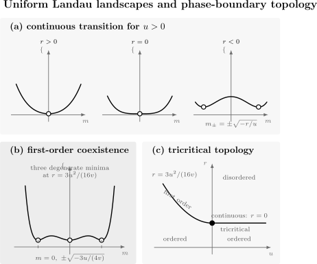
Uniform scalar Landau theory. For $u>0$, changing the quadratic coefficient through $r=0$ converts one symmetric minimum into two symmetry-related minima continuously. For $u<0$ and $v>0$, the first-order coexistence point has three degenerate minima. In the $(u,r)$ plane, the continuous line $r=0$ for $u>0$ and the coexistence curve $r=3u^2/(16v)$ for $u<0$ meet at the tricritical point.

Multicomponent Order Parameters

Landau theory is not restricted to one scalar. The main new task is to enumerate invariant tensors and test stability in every direction.

Quadratic form and the soft mode

Near the symmetric state, write

$$\mathcal f = \mathcal f_0 +\frac12 \sum_{a,b} \phi_a R_{ab} \phi_b +O(\phi^3),$$

with a symmetric Hessian

$$R_{ab} = R_{ba}.$$

Diagonalize $R$. A conventional continuous instability begins when its smallest eigenvalue passes through zero while the others remain positive.

If $\boldsymbol e_0$ is the soft eigenvector,

$$\boldsymbol\phi = \varphi\boldsymbol e_0 +\text{massive components}.$$

The quartic potential projected along $\boldsymbol e_0$ must be positive for the simplest continuous scenario. If several eigenvalues vanish together, a multicomponent critical subspace and additional tuning or symmetry are involved.

Massive components can shift coefficients

Suppose a noncritical variable $q$ couples as

$$\begin{aligned} \mathcal f(m,q) ={}& \frac r2m^2 +\frac u4m^4 \\ &+ \frac K2q^2 +\lambda q m^2, \\ & K>0. \end{aligned}$$

Minimizing over $q$ gives

$$q_\star = -\frac{\lambda}{K}m^2.$$

Substitution produces

$$\mathcal f_{\mathrm{eff}}(m) = \frac r2m^2 +\frac14 \left( u-\frac{2\lambda^2}{K} \right) m^4.$$

A secondary massive mode can therefore drive the effective quartic coefficient negative. “Integrating out” is harmless only after checking the induced terms and the scale separation.

Two competing scalar orders

For two inversion-symmetric orders $\phi$ and $\psi$, consider

$$\begin{aligned} \mathcal f ={}& \frac{r_\phi}{2}\phi^2 +\frac{u_\phi}{4}\phi^4 \\ &+ \frac{r_\psi}{2}\psi^2 +\frac{u_\psi}{4}\psi^4 +\frac w2\phi^2\psi^2. \end{aligned}$$

Assume

$$u_\phi>0, \qquad u_\psi>0.$$

When both orders are nonzero, stationarity gives

$$\begin{pmatrix} u_\phi & w \\ w & u_\psi \end{pmatrix} \begin{pmatrix} \phi^2 \\ \psi^2 \end{pmatrix} = - \begin{pmatrix} r_\phi \\ r_\psi \end{pmatrix}.$$

The determinant

$$D := u_\phi u_\psi-w^2$$

organizes the local mixed solution.

• If $D>0$ and the resulting $\phi^2,\psi^2$ are positive, a stable coexistence phase is possible.
• Strong positive $w$ favors competition and can replace coexistence by a first-order boundary between pure ordered phases.
• If $w<-\sqrt{u_\phi u_\psi}$, the quartic form is unstable along a mixed direction and higher powers are required.

The words bicritical, tetracritical, and multicritical require the full phase-boundary topology and tuning count, not just the presence of two order parameters.

Competing Orders carries this coupled potential into coexistence diagnostics, multicritical phase diagrams, fluctuation caveats, and material case studies.

Accidental degeneracy

If coefficients happen to enlarge the symmetry of the polynomial, a continuous manifold of minima can appear that is not protected by the microscopic symmetry. Higher-order invariants, fluctuations, or perturbations can lift this accidental degeneracy.

Emergent Symmetry owns the stronger claim that a larger symmetry governs the long-distance theory. Equality of two bare coefficients is not sufficient evidence.

Landau Theory and Mean-Field Theory

The terms are closely related but not identical.

Landau theory is phenomenological

Landau theory begins with:

1. an order parameter;
2. its symmetry representation;
3. an analytic invariant expansion;
4. minimization.

Its coefficients can be fitted, inferred from a microscopic calculation, or treated as smooth phenomenological functions of controls.

Mean field is a method

Microscopic mean-field theory begins with a Hamiltonian and approximates interactions through factorization, restricted variation, or a saddle point. When its thermodynamic functional is expanded near a transition, it often produces a Landau polynomial.

For example, a microscopic self-consistency equation can have the form

$$m = \mathcal G(m;T,h).$$

Expanding near $m=0$ can yield

$$0 = rm +um^3 -h +\cdots,$$

which is the stationarity equation of a Landau potential if the closure is thermodynamically integrable.

Shared exponents do not imply shared microscopics

Many unrelated mean-field models produce

$$\beta=\frac12, \qquad \gamma=1, \qquad \delta=3$$

because the same analytic quartic normal form controls their minima. These powers diagnose the approximation class, not the microscopic Hamiltonian.

Not every self-consistency equation has a valid potential

An iterative closure may produce fixed points without descending from a thermodynamic functional. Stability of the iteration map is then not the same as thermodynamic stability.

One must distinguish:

• convergence of a numerical iteration;
• positive curvature of a proposed potential;
• global minimum among candidate branches;
• stability against fluctuations outside the trial space.

Representative Physical Uses

Landau theory is a template rather than one model.

Ising-like magnet

For a magnetization $m$ at zero magnetic field,

$$m\mapsto-m$$

forbids odd terms. The scalar quartic theory captures the topology of a paramagnet-to-ferromagnet transition at mean-field level.

The Transverse-Field Ising Model owns the quantum lattice model and its actual critical behavior.

Liquid–gas critical endpoint

Density is not microscopically odd under an exact $Z_2$ symmetry. Near a critical endpoint, one can often define mixed temperature-like and ordering-field variables and shift the density so the leading normal form becomes Ising-like.

This emergent local structure does not mean liquid and gas are exchanged by an exact microscopic symmetry. Field mixing and analytic backgrounds matter when comparing amplitudes.

Superfluid or superconducting amplitude

A complex order parameter $\psi$ gives a uniform potential

$$\mathcal f = \mathcal f_0 +r\lvert\psi\rvert^2 +\frac u2\lvert\psi\rvert^4 +\cdots.$$

This predicts the equilibrium amplitude at saddle level. Gauge invariance, phase stiffness, vortices, electromagnetic fields, and number-conserving definitions require more structure than this uniform polynomial. Ginzburg–Landau Theory owns the superconducting material extension.

Structural and nematic transitions

Displacement modes, strain tensors, and orientational tensors transform under spatial point groups. Their allowed cubic and quartic invariants can predict:

• which ordered patterns are symmetry-compatible;
• whether several variants are degenerate;
• whether a simple continuous transition is allowed at polynomial level;
• which external stresses or fields split the variants.

The result depends on the full representation, not only the number of components.

Quantum transitions

At zero temperature, a static Landau potential can organize uniform ground-state phases as a coupling is varied. It does not determine:

• the imaginary-time kinetic term;
• the dynamical exponent $z$;
• coupling to gapless fermions or gauge modes;
• Berry phases;
• whether a local order-parameter-only action exists.

Quantum Phase Transitions owns the quantum-critical scaling framework.

What Landau Theory Predicts Reliably

When its assumptions hold, Landau theory can robustly predict:

• which polynomial terms symmetry permits;
• the number and symmetry relation of uniform minima;
• qualitative phase-boundary topology;
• whether a cubic invariant obstructs the simplest continuous transition;
• whether a quartic coefficient must be stabilized by sixth order;
• source-induced selection and rounding;
• mean-field equations of state and amplitude relations;
• the number of controls required to reach ordinary or multicritical points;
• candidate metastable branches within a uniform approximation.

Coefficient values, transition temperatures, and barrier heights remain nonuniversal.

Limitations and Breakdown

Landau theory is a controlled normal form only when the retained variables and analytic expansion are adequate.

Critical fluctuations

Near a continuous transition, the correlation length grows and fluctuations occur on many scales. Uniform minimization neglects their feedback.

For a short-range scalar $\phi^4$ theory, the quartic interaction is marginal at

$$d_c=4.$$

Above $d_c$, mean-field exponents generally apply with qualifications about dangerous irrelevance. Below $d_c$, fluctuations usually produce non-mean-field exponents. At $d_c$, logarithmic corrections can appear.

Low-dimensional continuous symmetry

A uniform potential can predict an ordered minimum for an $O(n)$ order parameter in situations where long-wavelength fluctuations forbid finite-temperature long-range order.

For short-range systems with continuous symmetry, Mermin–Wagner-type results rule out conventional spontaneous order in one and two spatial dimensions under their hypotheses. A Berezinskii–Kosterlitz–Thouless transition can occur without the ordinary Landau order-parameter power law.

Other soft modes

If the order parameter couples to another gapless field, integrating out that field can generate:

• nonanalytic powers;
• nonlocal interactions;
• singular damping;
• fluctuation-induced first-order behavior;
• more than one relevant slow variable.

The Halperin–Lubensky–Ma mechanism is a standard example in which gauge-field fluctuations can alter the transition predicted by a simple order-parameter potential. Metallic quantum critical points provide further cases where soft fermionic modes obstruct a local analytic order-parameter-only expansion.

Topological and nonlocal order

Some phases are distinguished by long-range entanglement, anyonic excitations, topological response, or nonlocal operators rather than a local symmetry-breaking order parameter. A local polynomial in $m$ is then not a complete classifier.

Deconfined and unconventional criticality

A continuous transition can involve fractionalized degrees of freedom, emergent gauge fields, or anomalies not visible in a polynomial of either adjacent phase’s conventional order parameter. Failure of the Landau description does not imply absence of a transition.

Disorder and rare regions

Quenched disorder can:

• randomize local coefficients;
• smear or round transitions under specified conditions;
• generate Griffiths regimes;
• change the fixed point;
• produce broad distributions not summarized by one uniform $m$.

Replacing a random coefficient by its average can erase the phenomenon of interest.

Exact convexity and phase coexistence

The exact Legendre-transformed equilibrium effective potential is convex under standard thermodynamic conditions. A nonconvex double-well polynomial should therefore be interpreted as a constrained, coarse-grained, or branch-resolved potential before complete phase separation and convexification.

At coexistence in the thermodynamic limit, the convex equilibrium construction can contain a flat segment corresponding to mixtures of phases. The nonconvex polynomial remains useful for identifying pure-phase minima and approximate barriers, but the two objects must not be conflated.

Dynamics and nucleation

Static Landau theory does not specify an equation of motion. Postulating

$$\partial_t m \propto -\frac{\partial\mathcal f}{\partial m}$$

adds kinetic assumptions that depend on conservation laws, reversible couplings, noise, and the environment.

Likewise, a uniform barrier does not determine a nucleation rate. Interfaces, droplets, surface tension, dissipation, and stochastic dynamics are required.

Polynomial truncation

The expansion is local in order-parameter space. Large minima can lie outside its radius of usefulness.

A trustworthy truncation checks:

• stability under adding the next allowed term;
• sensitivity of minima to coefficient uncertainty;
• whether the predicted order parameter remains small;
• whether omitted fields are actually massive;
• whether nonanalytic terms are expected.

A Reliable Landau Workflow

1. Fix the ensemble. Name the thermodynamic potential and controlled variables.
2. Define the order parameter. State operator, normalization, components, wavevector, and physical units.
3. State the symmetry action. Give how every component transforms at zero source.
4. List invariants systematically. Include all terms through a declared order.
5. Add sources with signs. Record the conjugate response convention.
6. Declare the expansion point. Identify the candidate critical or multicritical controls.
7. Test boundedness. Check the highest retained terms in every direction.
8. Find all stationary points. Do not stop at the first self-consistent solution.
9. Classify local stability. Evaluate the Hessian at each stationary point.
10. Compare global potentials. Locate coexistence by equal minima, not by hysteresis.
11. Derive observables. Differentiate the minimized potential while retaining coefficient dependence.
12. Audit fluctuations and omitted modes. Check dimension, interaction range, conservation laws, disorder, and other soft fields.
13. Separate prediction levels. Label symmetry consequences, Landau-level results, microscopic inputs, and RG-corrected statements.
14. Benchmark. Compare against an exact limit, microscopic mean field, simulation, experiment, or known universality class.

Common Mistakes

Expanding before defining the order parameter

The allowed terms depend on the representation, wavevector, and source convention.

Calling the polynomial the exact free energy

The off-shell Landau potential, constrained rate function, and minimized equilibrium free energy are related but distinct.

Dropping an allowed cubic invariant

Its absence requires symmetry or an explicit tuning argument.

Assuming no cubic term guarantees continuity

A negative quartic coefficient, coupling to another mode, or fluctuations can still produce first order.

Keeping a negative quartic without stabilization

If $u<0$, the quartic truncation is unbounded and cannot define equilibrium.

Identifying a spinodal with coexistence

Coexistence is equality of global minima. A spinodal is loss of local stability within an approximation.

Reporting mean-field exponents as exact

Their validity depends on dimension, range, fixed point, and the absence of singular extra modes.

Using iteration stability as thermodynamic stability

A convergent fixed-point algorithm need not minimize the correct potential.

Ignoring regular backgrounds

Heat capacities and susceptibilities can contain large analytic contributions that obscure the singular Landau piece.

Forgetting coefficient conventions

Changing $u m^4/4$ to $u m^4/4!$ changes every formula involving $u$.

Inferring dynamics from a static landscape

Relaxation laws and nucleation rates need independent kinetic input.

Treating every phase as Landau-classifiable

Topological order and unconventional critical points can lie outside local symmetry-breaking theory.

Exercises

Exercise 1: Continuous scalar minima

Consider

$$\mathcal f(m) = \frac r2m^2 +\frac u4m^4, \qquad u>0.$$

Find every stationary point, classify its local stability for $r>0$, $r=0$, and $r<0$, and compute the minimized potential.

Solution

Stationarity gives

$$\frac{d\mathcal f}{dm} = m(r+um^2) = 0.$$

Thus $m=0$ always exists, while

$$m_\pm = \pm\sqrt{-\frac r u}$$

exist only for $r<0$.

The curvature is

$$\mathcal f''(m) = r+3um^2.$$

For $r>0$, the origin has positive curvature and is the unique minimum. For $r=0$, the origin has zero quadratic curvature but the positive quartic term makes it a stable flat minimum. For $r<0$, the origin has negative curvature and is a maximum, while

$$\mathcal f''(m_\pm) = -2r >0,$$

so the two nonzero points are minima.

At either ordered minimum,

$$\begin{aligned} \mathcal f(m_\pm) &= \frac r2 \left( -\frac r u \right) +\frac u4 \left( \frac{r^2}{u^2} \right) \\ &= -\frac{r^2}{4u}. \end{aligned}$$

Therefore

$$f_{\mathrm{eq}} = \begin{cases} 0, &r\ge0, \\ -r^2/(4u), &r<0. \end{cases}$$

up to an additive analytic background.

Exercise 2: Mean-field exponents

For

$$h = rm+um^3, \qquad u>0,$$

derive $\beta$, $\gamma$, and $\delta$. State the paths used to define each exponent.

Solution

For $\beta$, set $h=0$ and approach from the ordered side $r\to0^-$:

$$m^2 = -\frac r u,$$

so

$$\lvert m\rvert \sim \lvert r\rvert^{1/2}$$

and

$$\beta=\frac12.$$

For $\gamma$, differentiate at fixed $r$:

$$\chi^{-1} = \frac{\partial h}{\partial m} = r+3um^2.$$

At $h\to0$ from $r>0$, $m=0$ and $\chi_+=1/r$. From $r<0$ on a selected ordered branch, $m^2=-r/u$ and

$$\chi_- = \frac{1}{2\lvert r\rvert}.$$

Both sides give

$$\gamma=1.$$

For $\delta$, set $r=0$ and approach $h\to0$:

$$m = \left( \frac h u \right)^{1/3},$$

with the real signed root understood. Thus

$$\delta=3.$$

Exercise 3: Susceptibility amplitude ratio

Let

$$r=at, \qquad a>0,$$

where $t$ is a reduced temperature. Show that the scalar quartic Landau model predicts

$$\frac{\Gamma_+}{\Gamma_-} = 2.$$

Which assumptions enter this number?

Solution

Above the transition,

$$\chi_+ = \frac{1}{at}, \qquad t>0,$$

so

$$\Gamma_+ = \frac1a.$$

Below the transition,

$$\chi_- = \frac{1}{2a\lvert t\rvert},$$

so

$$\Gamma_- = \frac{1}{2a}.$$

Therefore

$$\frac{\Gamma_+}{\Gamma_-} = 2.$$

The result assumes the same analytic linear coefficient $r=at$ on both sides, the normalization $u m^4/4$, a scalar $Z_2$ order parameter, uniform saddle-level minimization, and no fluctuation renormalization or field mixing. Changing the order-parameter normalization changes the individual amplitudes but not this ratio within the same scalar Landau convention.

Exercise 4: Sextic coexistence

For

$$\mathcal f(m) = \frac r2m^2 +\frac u4m^4 +\frac v6m^6,$$

with $u<0$ and $v>0$, derive the coexistence value of $r$ and the jump in $\lvert m\rvert$.

Solution

For a nonzero stationary point, set $x=m^2$:

$$r+ux+vx^2 = 0.$$

At coexistence with the $m=0$ minimum,

$$\frac r2x +\frac u4x^2 +\frac v6x^3 = 0.$$

Use

$$r = -ux-vx^2$$

from stationarity. Substitution gives

$$-\frac u4x^2 -\frac v3x^3 = 0.$$

For $x>0$,

$$x = -\frac{3u}{4v}.$$

Therefore

$$m_{\mathrm{coex}}^2 = -\frac{3u}{4v}.$$

Returning to the stationarity equation,

$$r_{\mathrm{coex}} = \frac{3u^2}{16v}.$$

The order parameter jumps from zero to

$$\lvert m_{\mathrm{coex}}\rvert = \sqrt{ -\frac{3u}{4v} }.$$

Exercise 5: Tricritical exponents

At

$$u=0, \qquad v>0,$$

use

$$\mathcal f(m) = \frac r2m^2 +\frac v6m^6 -hm$$

to derive the tricritical mean-field values of $\beta$, $\gamma$, $\delta$, and $\alpha$.

Solution

At $h=0$ and $r<0$,

$$r+vm^4 = 0,$$

so

$$\lvert m\rvert \sim \lvert r\rvert^{1/4}$$

and

$$\beta_{\mathrm t} = \frac14.$$

At $r=0$,

$$h = vm^5,$$

which gives

$$\delta_{\mathrm t} = 5.$$

The inverse susceptibility is

$$\chi^{-1} = r+5vm^4.$$

It equals $r$ above and $4\lvert r\rvert$ below, so

$$\gamma_{\mathrm t} = 1.$$

At the ordered minimum,

$$\lvert m\rvert^2 = \sqrt{ \frac{\lvert r\rvert}{v} },$$

and

$$f_{\mathrm s} = -\frac{\lvert r\rvert^{3/2}} {3\sqrt v}.$$

If $r\propto t$, then two temperature derivatives give

$$C_{\mathrm s} \sim \lvert t\rvert^{-1/2},$$

so

$$\alpha_{\mathrm t} = \frac12.$$

Exercise 6: Symmetry audit

For each order parameter, list the lowest nonconstant invariants through fourth order:

1. a real scalar with $Z_2$ symmetry;
2. a complex scalar with $U(1)$ symmetry;
3. a two-component vector with only independent sign flips and component exchange;
4. a traceless symmetric $3\times3$ tensor under rotations.

Solution

For a real $Z_2$ scalar $m$, the invariants are

$$m^2, \qquad m^4.$$

Odd powers are forbidden.

For a complex $U(1)$ scalar $\psi$, the invariants are

$$\lvert\psi\rvert^2, \qquad \lvert\psi\rvert^4.$$

Terms such as $\psi^2+\psi^{*2}$ are not $U(1)$ invariant.

For $\boldsymbol\phi=(\phi_x,\phi_y)$ with independent sign flips and exchange, two quartic structures are allowed:

$$\left( \phi_x^2+\phi_y^2 \right)^2$$

and

$$\phi_x^4+\phi_y^4.$$

The second distinguishes the discrete symmetry from full $O(2)$ invariance.

For a traceless symmetric tensor $Q$, the low invariants include

$$\operatorname{Tr}Q^2, \qquad \operatorname{Tr}Q^3,$$

and quartic combinations built from

$$\left( \operatorname{Tr}Q^2 \right)^2$$

and, depending on dimension and identities, $\operatorname{Tr}Q^4$. The allowed cubic invariant means that the simplest scalar $Z_2$ logic does not apply.

Exercise 7: Eliminating a secondary mode

Given

$$\begin{aligned} \mathcal f(m,q) ={}& \frac r2m^2 +\frac u4m^4 \\ &+ \frac K2q^2 +\lambda q m^2, \\ & K>0. \end{aligned}$$

eliminate $q$ by minimization. Under what condition does the resulting quartic theory remain stable?

Solution

Stationarity in $q$ gives

$$Kq+\lambda m^2 = 0,$$

so

$$q_\star = -\frac{\lambda}{K}m^2.$$

The $q$-dependent terms become

$$\begin{aligned} \frac K2q_\star^2 +\lambda q_\star m^2 &= \frac{\lambda^2}{2K}m^4 -\frac{\lambda^2}{K}m^4 \\ &= -\frac{\lambda^2}{2K}m^4. \end{aligned}$$

Thus

$$\mathcal f_{\mathrm{eff}}(m) = \frac r2m^2 +\frac14 \left( u-\frac{2\lambda^2}{K} \right) m^4.$$

The quartic truncation remains bounded when

$$u_{\mathrm{eff}} := u-\frac{2\lambda^2}{K} >0.$$

If $u_{\mathrm{eff}}<0$, sixth-order stabilization or a more complete treatment is required. The secondary mode can therefore change the predicted order of the transition even though it is noncritical by itself.

Exercise 8: Diagnose the limits of a Landau claim

A two-dimensional short-range quantum magnet at nonzero temperature has an exact continuous spin-rotation symmetry. A uniform saddle calculation finds a nonzero vector minimum and reports a conventional continuous transition with $\beta=1/2$.

Identify what is valid in the calculation and what has not been established.

Solution

The calculation can validly identify:

• the symmetry-allowed uniform invariants;
• the candidate ordered directions within the saddle approximation;
• the mean-field instability of the uniform potential;
• the exponent produced by that approximation.

It has not established a true finite-temperature phase transition with long-range vector order. For short-range interactions and exact continuous symmetry in two dimensions, long-wavelength fluctuations fall under Mermin–Wagner-type restrictions. The uniform calculation omits precisely those spatial fluctuations.

Depending on the symmetry and defects, the system may:

• have no finite-temperature transition;
• exhibit a Berezinskii–Kosterlitz–Thouless transition with algebraic order;
• acquire conventional order only after anisotropy, long-range interactions, interlayer coupling, or explicit symmetry breaking is included.

The reported $\beta=1/2$ is therefore a Landau-level result, not evidence for the claimed bulk universality class.

Key Takeaways

• Landau theory expands a uniform off-shell potential in symmetry-allowed order-parameter invariants and minimizes it.
• The order parameter, ensemble, source convention, and expansion point must be specified before coefficients have meaning.
• For a scalar $Z_2$ potential with $u>0$, $r=0$ gives a continuous mean-field transition with $\beta=1/2$, $\gamma=1$, $\delta=3$, and $\alpha=0$.
• A nonzero source tilts the potential and rounds the zero-source critical singularity along a generic path.
• A symmetry-allowed cubic term generically favors first order at polynomial level.
• With $u<0$ and $v>0$, coexistence occurs at $r=3u^2/(16v)$ and $m^2=-3u/(4v)$.
• The point $r=u=0$, $v>0$ is tricritical and requires two tunings.
• Multicomponent problems are controlled by invariant tensors, Hessian eigenmodes, and couplings among order parameters.
• Landau theory and microscopic mean-field theory often meet at the same polynomial but are not synonymous.
• Critical fluctuations, low dimension, gapless extra modes, disorder, and topological structure can invalidate a local analytic order-parameter-only description.

Further Reading

• For microscopic decoupling and self-consistency, see Mean-Field Theory.
• For exact equilibrium potentials and coexistence, see Thermodynamic Potentials.
• For bulk evidence distinguishing first-order and continuous transitions, see Finite-Temperature Phase Transitions.
• For the exponent dictionary and data analysis, see Critical Exponents and Scaling.
• For why fluctuations change the simple polynomial predictions, see Renormalization Group Preview.
• For order-parameter representations and nonlocal alternatives, see Order Parameters.
• For the magnetic double well in a material setting, including domains, Curie behavior, and the limits of equilibrium Landau theory for hysteresis, see Ferromagnetism.

References

• L. D. Landau, “The Theory of Phase Transitions”, Nature 138, 840–841, 1936.
• L. D. Landau, “On the Theory of Phase Transitions”, in Collected Papers of L. D. Landau, pp. 193–216, Pergamon, 1965; original work published in 1937.
• P. M. Chaikin and T. C. Lubensky, Principles of Condensed Matter Physics, Cambridge University Press, 1995.
• N. Goldenfeld, Lectures on Phase Transitions and the Renormalization Group, CRC Press reissue.
• M. Kardar, Statistical Physics of Fields, Cambridge University Press, 2007.
• J. P. Sethna, Statistical Mechanics: Entropy, Order Parameters, and Complexity, 2nd ed., Oxford University Press, 2021.
• K. G. Wilson and J. Kogut, “The Renormalization Group and the $\epsilon$ Expansion”, Physics Reports 12, 75–199, 1974.
• M. E. Fisher, “The Renormalization Group in the Theory of Critical Behavior”, Reviews of Modern Physics 46, 597–616, 1974.
• K. G. Wilson, “The Renormalization Group: Critical Phenomena and the Kondo Problem”, Reviews of Modern Physics 47, 773–840, 1975.
• H. E. Stanley, “Scaling, Universality, and Renormalization: Three Pillars of Modern Critical Phenomena”, Reviews of Modern Physics 71, S358–S366, 1999.
• N. D. Mermin and H. Wagner, “Absence of Ferromagnetism or Antiferromagnetism in One- or Two-Dimensional Isotropic Heisenberg Models”, Physical Review Letters 17, 1133–1136, 1966.
• P. C. Hohenberg, “Existence of Long-Range Order in One and Two Dimensions”, Physical Review 158, 383–386, 1967.
• B. I. Halperin, T. C. Lubensky, and S.-K. Ma, “First-Order Phase Transitions in Superconductors and Smectic-A Liquid Crystals”, Physical Review Letters 32, 292–295, 1974.
• D. Belitz, T. R. Kirkpatrick, and T. Vojta, “How Generic Scale Invariance Influences Quantum and Classical Phase Transitions”, Reviews of Modern Physics 77, 579–632, 2005.
• H. Touchette, “The Large Deviation Approach to Statistical Mechanics”, Physics Reports 478, 1–69, 2009.
• M. Blume, “Theory of the First-Order Magnetic Phase Change in UO$_2$”, Physical Review 141, 517–524, 1966.
• H. W. Capel, “On the Possibility of First-Order Phase Transitions in Ising Systems of Triplet Ions with Zero-Field Splitting”, Physica 32, 966–988, 1966.
• K. Binder, “Theory of First-Order Phase Transitions”, Reports on Progress in Physics 50, 783–859, 1987.