Order Parameters

An order parameter is a macroscopic variable chosen to distinguish phases or symmetry-related thermodynamic states. In the standard symmetry-breaking setting, it is built from an operator that transforms nontrivially under a symmetry and acquires a definite value in a selected ordered state.

The short slogan

$$\begin{gathered} \text{ordered phase} \\ \Longleftrightarrow \\ \text{nonzero order parameter} \end{gathered}$$

is useful only after several qualifications:

• the operator and its normalization must be specified;
• the spatial wavevector or form factor may be essential;
• a finite symmetry eigenstate can have zero one-point value even when its correlations reveal order;
• a condensate or pair amplitude can vanish in a fixed-number description;
• a response coefficient, excitation gap, mean field, and order parameter are different objects;
• some phases have no local Landau order parameter;
• a gauge-dependent amplitude is not itself a gauge-invariant observable.

Order parameters are therefore structured diagnostics, not universal labels attached to phases without a state, limit, symmetry, or measurement prescription.

Canonical Scope

This page is the canonical home for the general many-body language of order parameters. It owns:

• the passage from a microscopic operator to an extensive ordering mode and an intensive macroscopic value;
• symmetry transformation laws and order-parameter components;
• conjugate sources and source-selected limits;
• one-point, squared-order, correlation, and structure-factor diagnostics;
• uniform magnetization, staggered magnetization, condensate amplitude, pairing amplitude, and density-wave order as representative examples;
• the distinction between local, composite, bilocal, string, loop, and topological diagnostics;
• normalization, finite-size, experimental, and numerical failure modes.

Neighboring pages retain separate ownership:

• Emergence and Effective Degrees of Freedom owns cross-mechanism variable selection, observable matching, error, and breakdown audits; this page retains order-parameter construction, source and state-selection limits, and phase-specific diagnostics.
• Phases of Matter in Many-Body QM owns the broader definition and multi-diagnostic fingerprint of a phase.
• Thermodynamic Limit owns limiting sequences, boundary conditions, and noncommuting bulk limits.
• Spontaneous Symmetry Breaking owns Hamiltonian versus state symmetry, source-selected phases, finite-size cat states, and tower spectra.
• Long-Range Order owns pointwise correlation limits, their volume-averaged form, and extensive peak scaling.
• Off-Diagonal Long-Range Order owns reduced-density-matrix eigenvalue criteria for bosonic and fermion-pair condensates.
• Connected Correlation Functions owns cluster decomposition, pure-phase selection, and connected subtraction.
• Structure Factors owns static and dynamic momentum-space correlation conventions.
• Susceptibilities owns the source–detector response dictionary and order-of-limits distinctions.
• Mean-Field Theory owns self-consistency, channel selection, variational bounds, and saddle stability.
• Landau Theory owns symmetry-allowed uniform potentials, minimization, mean-field exponents, and tricriticality.
• Landau–Ginzburg Theory Preview owns coarse-grained spatial fields, gradient stiffness, Gaussian correlation lengths, and interfaces.
• Bose–Einstein Condensation owns the Penrose–Onsager criterion, condensate fraction, and ideal-gas benchmark.
• BCS Mean-Field Theory owns anomalous decoupling, the gap equation, coherence factors, and number projection.
• Topological Invariants owns the mathematical definition and limitations of invariant-based classification.

The examples here explain what the variables mean. Model pages retain their phase diagrams and exact formulas.

Three Layers of the Definition

An order parameter is easiest to audit when three layers are kept separate.

Microscopic operator

Choose local or finitely supported operators

$$\widehat o_a(\mathbf r),$$

where $a$ labels spin components, orbitals, sublattices, pair channels, or another internal structure.

The microscopic operator fixes:

• units;
• Hermiticity or complex character;
• locality and support;
• transformation under internal and spatial symmetries;
• what an external source would couple to;
• which experimental probe can access the channel.

Extensive ordering mode

Project the microscopic field into a spatial pattern. On a lattice with $N$ sites, a common definition is

$$\widehat M_a(\mathbf Q) = \sum_{j=1}^{N} f_j(\mathbf Q)\, \widehat o_{a,j}.$$

For a simple Fourier mode,

$$f_j(\mathbf Q) = e^{-i\mathbf Q\cdot\mathbf r_j}.$$

Uniform order uses $\mathbf Q=\mathbf0$. Antiferromagnetic or density-wave order generally uses a nonzero ordering wavevector. Bond, orbital, and multipolar order may require matrix-valued or direction-dependent form factors rather than a scalar Fourier phase.

Intensive macroscopic value

The order parameter is usually the intensive selected-state limit

$$\phi_a(\mathbf Q) = \lim_{N\to\infty} \frac{1}{N} \left\langle \widehat M_a(\mathbf Q) \right\rangle_{\mathrm{sel}}.$$

For a continuum system, $N^{-1}$ may be replaced by $V^{-1}$, or the field itself may already be a density. The convention must be stated because an extensive $\langle\widehat M\rangle$, an intensive $\phi$, and a Fourier transform normalized by $1/\sqrt N$ have different size scaling.

The subscript “sel” is not decorative. It records a symmetry-breaking source, boundary condition, phase sector, measurement conditioning, or another prescription that selects one macroscopic state.

Symmetry Transformation

Let $G$ be a symmetry group represented by $U(g)$. A set of candidate operators forms a representation when

$$\begin{aligned} U(g)^\dagger \widehat o_a(\mathbf r) U(g) ={}& \sum_b D_{ab}(g)\, \widehat o_b(g^{-1}\mathbf r). \end{aligned}$$

The spatial argument is absent for a purely internal symmetry. For a selected state, the corresponding order-parameter components transform schematically as

$$\boldsymbol\phi \longmapsto D(g)\boldsymbol\phi,$$

with an additional wavevector phase for translations.

If

$$D(g)\boldsymbol\phi = \boldsymbol\phi,$$

then $g$ belongs to the unbroken subgroup $H$. A symmetry-breaking pattern is summarized by

$$G \longrightarrow H.$$

The orbit of symmetry-related order-parameter values is often the coset space

$$\mathcal M_{\mathrm{OP}} \simeq G/H.$$

This statement is local and symmetry based. It does not by itself classify topological sectors, defects, amplitudes that can vanish, or disconnected pieces generated by extra microscopic constraints.

Representative geometries

Symmetry pattern	Order parameter	Symmetry-related values
Ising $\mathbb Z_2$	real scalar $m$	$m=\pm m_0$
planar spin rotation	two-component vector	circle of directions
three-dimensional spin rotation	three-component vector	sphere of directions
global particle-number $U(1)$	complex amplitude $\Phi$	phase circle at fixed magnitude
period-$p$ translation breaking	complex density-wave amplitude	$p$ commensurate phases
nematic rotation breaking	traceless tensor $Q_{ab}$	symmetry-related principal axes

The number of components is not the number of phases. Components describe coordinates; disconnected minima and residual identifications determine the symmetry-related states.

Conjugate Sources

A source makes the operational meaning explicit. For Hermitian channels,

$$\begin{aligned} H[\mathbf h] = H_0 - \sum_a \int d^d r\, h_a(\mathbf r)\, \widehat o_a(\mathbf r). \end{aligned}$$

For a complex field $\Phi$ with source $\eta$, Hermiticity requires

$$H_\eta = H_0 - \int d^d r\, \left( \eta^*\widehat\psi + \eta\widehat\psi^\dagger \right).$$

At positive temperature, the free energy

$$F[\mathbf h] = -\frac{1}{\beta} \ln \operatorname{Tr} e^{-\beta H[\mathbf h]}$$

generates the expectation value. For a uniform extensive source,

$$\phi_a = -\frac{1}{V} \frac{\partial F}{\partial h_a}.$$

The static susceptibility is a further derivative:

$$\chi_{ab} = \frac{\partial\phi_a}{\partial h_b}.$$

Thus the order parameter, source, and susceptibility have different units and physical roles:

$$\begin{gathered} \text{source} \\ \longrightarrow \\ \text{state response} \\ \longrightarrow \\ \text{order parameter}. \end{gathered}$$

A large susceptibility indicates a strong ordering tendency. It does not by itself prove a nonzero thermodynamic order parameter.

The Source-Selected Limit

Suppose $\widehat M$ is odd under an exact symmetry. At every finite $N$, a unique symmetry eigenstate generally has

$$\langle\widehat M\rangle_{N,0} = 0.$$

The broken-symmetry value is instead characterized by an ordered limit such as

$$m = \lim_{h\to0^+} \lim_{N\to\infty} \frac{1}{N} \langle\widehat M\rangle_{N,h}.$$

Reversing the limits can give

$$\lim_{N\to\infty} \lim_{h\to0} \frac{1}{N} \langle\widehat M\rangle_{N,h} = 0.$$

The source direction chooses a branch. For a vector order parameter, one may write

$$\mathbf h = h\,\widehat{\mathbf n}, \qquad h\to0^+,$$

so the limiting state is selected along $\widehat{\mathbf n}$.

This construction is not the only possible phase-selection prescription. Fixed boundary spins, symmetry-breaking boundary fields, a chosen infinite-volume extremal state, or conditioning on a measurement outcome can play an analogous role. The prescription and order of limits must be reported.

What Finite Systems Can Show

A vanishing finite-size one-point function is often required by symmetry. Several symmetry-compatible quantities can still diagnose incipient order.

Squared order parameter

Define the intensive root-mean-square amplitude

$$m_{\mathrm{rms}}(N) = \frac{1}{N} \sqrt{ \left\langle \widehat M^\dagger\widehat M \right\rangle }.$$

If long-range order survives,

$$\lim_{N\to\infty} m_{\mathrm{rms}}(N) = m_0 > 0.$$

Short-range correlations usually give

$$\left\langle \widehat M^\dagger\widehat M \right\rangle = O(N),$$

so

$$m_{\mathrm{rms}}(N) = O(N^{-1/2}).$$

Structure-factor scaling

With

$$S_O(\mathbf Q) = \frac{1}{N} \left\langle \widehat M^\dagger(\mathbf Q) \widehat M(\mathbf Q) \right\rangle,$$

the squared amplitude obeys

$$m_{\mathrm{rms}}^2(N) = \frac{S_O(\mathbf Q)}{N}.$$

An ordered phase therefore has

$$S_O(\mathbf Q) \sim N m_0^2,$$

whereas a noncritical short-range-correlated phase normally has $S_O(\mathbf Q)=O(1)$.

Critical states, algebraic phases, conservation constraints, long-range interactions, and unusual geometries can produce intermediate scaling. A single size cannot distinguish these cases.

Full long-distance correlation

For a local scalar channel,

$$\lim_{|\mathbf r|\to\infty} \left\langle \widehat o(\mathbf r) \widehat o(\mathbf0) \right\rangle = m_0^2$$

is a long-range-order diagnostic. In a selected pure phase,

$$\langle\widehat o\rangle = m_0,$$

and the connected correlator subtracts the plateau:

$$\begin{aligned} \left\langle \widehat o(\mathbf r) \widehat o(\mathbf0) \right\rangle_c \longrightarrow 0. \end{aligned}$$

In a symmetric finite state or phase mixture, the one-point function can vanish while the full correlator retains the plateau. Connected subtraction must therefore be interpreted together with phase selection.

Probability distribution

Repeated measurements or Monte Carlo samples can estimate a distribution $P_N(m)$. An Ising-like ordered finite system may show two peaks near

$$m = \pm m_0$$

even when the mean vanishes. A broad single peak, a two-peak distribution, and a multi-component ring encode different order-parameter geometries.

Histograms depend on sampling dynamics, sector tunneling, estimator bias, and boundary conditions. They supplement rather than replace size scaling.

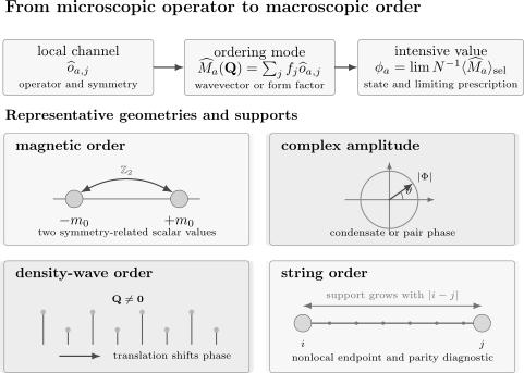
An order parameter requires an operator channel, a symmetry or spatial projection, and a macroscopic limiting prescription. Uniform magnetization, a complex condensate or pair amplitude, and density-wave order are local or finitely supported Landau channels. String order is nonlocal because its support grows with the endpoint separation.

A Practical Classification

Several independent adjectives are needed to describe an order parameter.

Question	Possibilities	Why it matters
spatial support	onsite, bond, plaquette, bilocal, string, loop	determines locality and accessible probes
symmetry type	scalar, vector, tensor, spinor, complex field	determines transformation law and allowed couplings
ordering wavevector	uniform or finite $\mathbf Q$	distinguishes ferroic and modulated patterns
microscopic content	spin, density, orbital, pair, bond, current	identifies the physical channel
Hermiticity	Hermitian or complex	fixes source terms and independent components
phase selection	source, boundary, sector, conditioning	fixes the thermodynamic state
diagnostic	one-point, squared, correlation, structure factor	controls finite-size interpretation
observability	direct, inferred, gauge fixed, response based	determines experimental meaning

These axes do not collapse into one label. A pairing field can be complex, bilocal in relative coordinate, local in its center-of-mass envelope, and gauge dependent. A density wave can be a local density channel but require a nonzero wavevector projection.

Magnetization

Magnetization is the cleanest prototype because the microscopic operator and symmetry action are visible.

Uniform ferromagnetic order

For $N$ localized spins, define

$$\widehat{\mathbf M} = \sum_{j=1}^{N} \widehat{\mathbf S}_j, \qquad \mathbf m = \lim_{N\to\infty} \frac{1}{N} \langle\widehat{\mathbf M}\rangle_{\mathrm{sel}}.$$

Under spin rotation $R$,

$$\mathbf m \longmapsto R\mathbf m.$$

Under time reversal,

$$\mathbf m \longmapsto -\mathbf m.$$

A nonzero $\mathbf m$ can therefore break spin rotation, time reversal, or both, depending on the Hamiltonian and whether spin–orbit coupling has already reduced the symmetry.

For an Ising magnet, only one component is active:

$$\widehat M_z = \sum_j \widehat S_j^z.$$

The symmetry sends

$$\widehat M_z \longmapsto -\widehat M_z,$$

and the ordered branches have $m_z=\pm m_0$. The Transverse-Field Ising Model gives the exact one-dimensional benchmark and its finite-size parity states.

Staggered antiferromagnetic order

Zero uniform magnetization does not imply absence of magnetic order. On a bipartite lattice, define

$$\widehat{\mathbf N} = \sum_j \eta_j\widehat{\mathbf S}_j, \qquad \eta_j = \begin{cases} +1,&j\in A,\\ -1,&j\in B. \end{cases}$$

The Néel order parameter is

$$\mathbf n = \lim_{N\to\infty} \frac{1}{N} \langle\widehat{\mathbf N}\rangle_{\mathrm{sel}}.$$

Equivalently, it is a spin mode at the antiferromagnetic wavevector $\mathbf Q_{\mathrm{AF}}$. A one-site translation can reverse $\mathbf n$, while spin rotations rotate its direction. The order therefore intertwines spatial and internal symmetry.

The XXZ Spin Chain shows how staggered order, a gapless liquid, and ferromagnetism occupy different anisotropy regimes.

Magnetization density and magnetic units

A condensed-matter magnetic moment density may include

$$\mathbf M_{\mathrm{phys}} = -g\mu_B \frac{1}{V} \sum_j \langle\widehat{\mathbf S}_j\rangle,$$

with signs, $g$ tensors, orbital moments, and unit-system factors. A dimensionless spin order parameter and SI magnetization are not interchangeable. The microscopic source coupling determines the correct normalization.

Condensate Amplitude

For a bosonic field, a broken-symmetry description introduces

$$\Phi(\mathbf r) = \left\langle \widehat\psi(\mathbf r) \right\rangle_{\mathrm{sel}}.$$

Under a global particle-number transformation,

$$\widehat\psi \longmapsto e^{i\theta}\widehat\psi,$$

so

$$\Phi \longmapsto e^{i\theta}\Phi.$$

The magnitude and phase can be written

$$\Phi(\mathbf r) = \sqrt{n_0(\mathbf r)}\, e^{i\vartheta(\mathbf r)}$$

within a weakly depleted symmetry-breaking description. The phase is defined relative to a reference, and gradients of it enter superfluid hydrodynamics.

Fixed-number caveat

If the state has exact particle number,

$$\widehat N \lvert\Psi_N\rangle = N \lvert\Psi_N\rangle,$$

then

$$\left\langle \Psi_N \middle| \widehat\psi \middle| \Psi_N \right\rangle = 0$$

because $\widehat\psi$ changes particle number. Condensation can nevertheless be present.

The number-conserving criterion uses the one-body density matrix

$$\gamma(\mathbf r,\mathbf r') = \left\langle \widehat\psi^\dagger(\mathbf r) \widehat\psi(\mathbf r') \right\rangle.$$

An eigenvalue proportional to $N$ identifies Bose–Einstein condensation without assuming $\Phi\ne0$.

The two descriptions can agree for suitable bulk observables in their common regime, but they answer different formal questions:

• $\Phi$ is a phase-selected anomalous one-point amplitude;
• the largest eigenvalue of $\gamma$ is number conserving;
• condensate fraction is an occupation ratio;
• superfluid stiffness is a response to a twist;
• long-range coherence is a correlation property.

None of these equalities is automatic in every dimension, temperature, interaction range, or nonequilibrium setting.

Lattice condensate field

For lattice bosons,

$$\psi_i = \langle \widehat b_i\rangle_{\mathrm{sel}}.$$

A uniform mean-field ansatz sets $\psi_i=\psi$, while a modulated condensate can carry finite momentum or sublattice structure. The Bose–Hubbard Model shows why a finite fixed-number system has $\langle b_i\rangle=0$ even when correlations and stiffness indicate a superfluid regime.

Pairing Amplitude

For fermionic fields, a pair amplitude is

$$F_{\alpha\beta} (\mathbf r,\mathbf r') = \left\langle \widehat\psi_\alpha(\mathbf r) \widehat\psi_\beta(\mathbf r') \right\rangle_{\mathrm{sel}}.$$

Fermi statistics requires

$$\begin{aligned} F_{\alpha\beta} (\mathbf r,\mathbf r') = - F_{\beta\alpha} (\mathbf r',\mathbf r). \end{aligned}$$

Under global particle-number $U(1)$,

$$F \longmapsto e^{2i\theta}F.$$

The factor of two records the particle number carried by the pair operator.

Gap function versus anomalous amplitude

For an interaction kernel $V$, a mean-field gap function can be defined schematically by

$$\begin{aligned} \Delta_{\alpha\beta} (\mathbf r,\mathbf r') = - \sum_{\gamma,\delta} V_{\alpha\beta;\gamma\delta} (\mathbf r,\mathbf r')\, F_{\gamma\delta} (\mathbf r,\mathbf r'). \end{aligned}$$

The pairing amplitude $F$, mean-field field $\Delta$, and minimum quasiparticle excitation gap are not generally the same object.

• $F$ is an anomalous expectation value.
• $\Delta$ includes the interaction kernel and channel convention.
• a spectral gap is an energy.
• nodes, anisotropy, strong coupling, disorder, competing orders, and frequency dependence can separate their magnitudes.

The equality between $|\Delta|$ and a simple spectral threshold belongs to restricted BCS models.

Relative and center-of-mass structure

Introduce

$$\mathbf R = \frac{\mathbf r+\mathbf r'}{2}, \qquad \boldsymbol\rho = \mathbf r-\mathbf r'.$$

The relative coordinate carries orbital and spin-pairing symmetry. The center-of-mass coordinate carries vortices, boundaries, pair-density waves, and long-wavelength textures.

A channel decomposition has the form

$$F(\mathbf R,\boldsymbol\rho) = \sum_\Gamma \Phi_\Gamma(\mathbf R)\, f_\Gamma(\boldsymbol\rho),$$

where $\Gamma$ labels symmetry channels. Calling a superconductor “$s$ wave” or “$d$ wave” is a statement about $f_\Gamma$ and the crystal symmetry, not merely about a nonzero scalar.

Number conservation and gauge caution

In a fixed-number state,

$$\langle \widehat\psi\widehat\psi \rangle = 0,$$

while pair correlations or a two-body reduced density matrix can still reveal pair condensation. The same logic that separates $\Phi$ from the one-body density matrix separates $F$ from number-conserving pair diagnostics.

For a charged superconductor, electromagnetic gauge transformations are a redundancy, not an ordinary physical global symmetry that can be diagnosed by a gauge-variant local observable. A gauge-fixed $\Delta$ is an efficient coordinate for calculations, while measurable statements involve gauge-invariant responses and relative phases, such as:

• magnetic flux expulsion;
• phase stiffness coupled to the gauge field;
• flux quantization;
• Josephson relations between two phase references;
• gauge-invariant correlation functions with appropriate parallel transport.

This caution does not make the BCS order parameter useless. It specifies how its phase and observability must be interpreted.

Density-Wave Order

A density wave modulates a conserved density without requiring a nonzero uniform density difference between phases. Define

$$\widehat\rho_{\mathbf Q} = \frac{1}{N} \sum_{j=1}^{N} e^{-i\mathbf Q\cdot\mathbf r_j} \left( \widehat n_j-\bar n \right).$$

The selected amplitude is

$$\rho_{\mathbf Q} = \lim_{N\to\infty} \left\langle \widehat\rho_{\mathbf Q} \right\rangle_{\mathrm{sel}}.$$

With this Fourier convention, a translation by $\mathbf a$ changes the amplitude by a phase of the form

$$\rho_{\mathbf Q} \longmapsto e^{i\mathbf Q\cdot\mathbf a} \rho_{\mathbf Q},$$

with the sign reversed if the opposite active-translation or Fourier convention is used.

The real-space modulation is

$$\delta n(\mathbf r) = \rho_{\mathbf Q} e^{i\mathbf Q\cdot\mathbf r} + \rho_{\mathbf Q}^* e^{-i\mathbf Q\cdot\mathbf r}.$$

For a period-two chain,

$$Q = \frac{\pi}{a},$$

and one-site translation sends $\rho_Q\to-\rho_Q$. The two signs label the two translated patterns.

Finite-size detector

A translation eigenstate can have

$$\langle\widehat\rho_{\mathbf Q}\rangle = 0.$$

The density structure factor

$$\begin{aligned} S_n(\mathbf Q) = \frac{1}{N} \sum_{j,k} e^{-i\mathbf Q\cdot(\mathbf r_j-\mathbf r_k)} \left\langle \delta\widehat n_j \delta\widehat n_k \right\rangle \end{aligned}$$

grows as $N|\rho_{\mathbf Q}|^2$ in a long-range-ordered phase, up to normalization and phase-selection details.

The half-filled Spinless Fermion Chains page provides a concrete charge-density-wave benchmark and its relation to staggered spin order.

Charge, spin, bond, and pair density waves

The modulated operator need not be particle density:

Pattern	Microscopic channel
charge-density wave	$\widehat n_j$
spin-density wave	$\widehat{\mathbf S}_j$
bond order	$\widehat c_i^\dagger\widehat c_j+\mathrm{h.c.}$
current order	$i(\widehat c_i^\dagger\widehat c_j-\mathrm{h.c.})$
pair-density wave	$\widehat c_i\widehat c_j$ in a finite-$\mathbf Q$ pair channel

Each has a different symmetry, source, and experimental vertex. A peak at the same $\mathbf Q$ does not make the channels equivalent.

Charge and Spin Density Waves applies this operator-first classification to nesting, Peierls physics, material probes, reconstruction, and collective modes.

Local and Composite Order

A local order parameter is built from an operator whose support remains bounded as the system grows. “Local” does not mean “onsite.”

• $\widehat S_j^z$ is onsite.
• $\widehat{\mathbf S}_i\cdot\widehat{\mathbf S}_{i+1}$ is a local bond operator.
• a plaquette current is local on a fixed loop.
• a pair operator on a fixed bond is composite but finitely supported.

Coarse graining can turn these microscopic objects into smooth fields

$$\phi_a(\mathbf r).$$

Their long-wavelength symmetry and component structure, rather than every lattice detail, enter a Landau description.

Composite does not mean nonlocal

An operator containing several microscopic factors can remain local:

$$\widehat B_i = \widehat{\mathbf S}_i \cdot \widehat{\mathbf S}_{i+1}.$$

Its support is one bond independent of system size. By contrast, a string whose length grows with endpoint separation is genuinely nonlocal.

Bilocal order

The anomalous pair field

$$F(\mathbf r,\mathbf r')$$

is bilocal in microscopic coordinates. If pair size remains finite, one can project its relative-coordinate structure into a local center-of-mass field $\Phi_\Gamma(\mathbf R)$. If pair correlations are extended or singular, that reduction requires care.

Locality is therefore a statement about the scale and representation being used.

Nonlocal Order Parameters

Some phases evade classification by local expectation values. Nonlocal diagnostics can expose hidden symmetry organization, confinement structure, or topology.

String order

For a spin chain, a representative string correlator is

$$\begin{aligned} \widehat X_{ij}^\alpha ={}& \widehat S_i^\alpha \exp\left( i\pi \sum_{k=i+1}^{j-1} \widehat S_k^\alpha \right) \\ &\times \widehat S_j^\alpha , \\ \mathcal O_{\mathrm{string}}^\alpha ={}& \lim_{|i-j|\to\infty} \left\langle \widehat X_{ij}^\alpha \right\rangle. \end{aligned}$$

The exponential records the parity of fluctuations between the endpoints. Its support grows with $|i-j|$, so it is not a local Landau field.

A nonzero value can diagnose hidden order in appropriate spin chains, but it is not a universal complete invariant. The result can depend on:

• which symmetry is imposed;
• endpoint operators;
• path or orientation;
• boundary conditions;
• whether perturbations preserve the protecting structure;
• the representation used.

Loop and membrane diagnostics

In gauge and topologically ordered systems, one may study operators supported on closed loops, open strings with endpoint excitations, or higher-dimensional membranes. Their scaling can distinguish regimes, but the interpretation depends on dimension, matter content, boundary conditions, and whether dynamical charges can screen the operator.

This page does not develop gauge-theory loop laws. The lesson is narrower:

$$\begin{gathered} \text{absence of local order} \\ \not\Longrightarrow \\ \text{absence of phase structure}. \end{gathered}$$

Topological data are not ordinary order parameters

A Chern number, anyon content, topological ground-state structure, or entanglement invariant can distinguish phases without a local symmetry-breaking field. These quantities are often called generalized order parameters in broad language, but they do not all behave like a local expectation value conjugate to a source.

Topological Order Preview explains how local indistinguishability, loop operators, anyons, and long-range entanglement replace a single local classifier in a conventional two-dimensional intrinsic topological phase.

It is safer to say exactly which object is used:

• local order parameter;
• nonlocal string or loop diagnostic;
• disorder operator;
• response invariant;
• entanglement diagnostic;
• topological invariant.

Symmetry-Protected Structure Preview explains why every protection statement must name the preserved symmetry, gap, locality class, and allowed deformation.

Locality Can Depend on Variables

A nonlocal transformation can exchange local and string-like operators. Under the Jordan–Wigner map, a local fermion operator contains a spin string, while fermion density maps to a local spin component.

Consequently:

• “local order” must name the microscopic variables;
• dual variables can turn an order operator into a disorder operator;
• an easy diagnostic in one representation can be nonlocal in another;
• locality of the Hamiltonian and locality of a chosen observable are separate questions.

The Jordan–Wigner Transformation owns the full spin–fermion dictionary and boundary-sector caveats.

Order Parameters and Mean Fields

A mean field is an expectation value introduced to simplify an interacting problem. It becomes an order parameter only if it distinguishes the relevant phases or symmetry-related states.

For example,

$$\bar n = \langle\widehat n_i\rangle$$

can be nonzero in every phase and merely set the density. By contrast,

$$\delta n_i = \langle\widehat n_i\rangle-\bar n$$

projected at a broken-translation wavevector can be a density-wave order parameter.

Likewise, a Hartree field, exchange field, anomalous pair field, and bond field may all appear in one self-consistent approximation. Whether any of them is an order parameter depends on:

• its symmetry;
• whether it vanishes in the comparison phase;
• whether the exact system supports the corresponding long-distance order;
• whether the approximation permits competing channels;
• whether the value survives the proper limit.

A nonzero saddle can be an artifact of a restricted ansatz, initialization, finite numerical precision, or omitted fluctuations. Mean-field self-consistency is evidence within an approximation, not a proof of exact order.

Order Parameter Versus Nearby Quantities

Quantity	Definition or role	Why it differs
order parameter	macroscopic phase-distinguishing variable	labels selected order
source	field linearly coupled to an operator	explicitly biases the state
susceptibility	derivative of a detector with respect to a source	measures response, not order itself
mean field	self-consistent approximation variable	may remain nonzero without symmetry distinction
spectral gap	energy to an excitation or sector	has energy units and need not track order uniquely
stiffness	free-energy cost of a twist or gradient	response coefficient
condensate fraction	macroscopic natural-orbital occupation divided by $N$	number-conserving occupation diagnostic
correlation length	scale of spatial decay	can grow without a nonzero one-point value
topological invariant	deformation-stable global datum	need not be a local expectation value

Several common comparisons follow.

Nonzero does not always mean ordered

The transverse magnetization in an Ising model can be nonzero on both sides of the transition because it is invariant under the broken $\mathbb Z_2$ symmetry. The particle density is normally nonzero in both a superfluid and a Mott phase.

Zero does not always mean disordered

A finite parity eigenstate, fixed-number condensate, translation eigenstate, or rotational singlet can have a vanishing one-point order parameter while squared amplitudes and correlations reveal the ordered thermodynamic structure.

A gap can close without being an order parameter

An excitation gap can vanish at a transition, throughout a stable gapless phase, or because of a symmetry-protected boundary mode. It is a spectral diagnostic, not an expectation value.

A stiffness can survive without true local long-range order

Low-dimensional systems can support algebraic order or a finite superfluid stiffness even when the one-point condensate amplitude vanishes in the symmetry-preserving thermodynamic description. Dimensionality and temperature must therefore accompany the claim.

Superfluidity in Condensed Matter applies the condensate-amplitude, ODLRO, and stiffness distinction to neutral-material evidence; this page retains the general order-parameter taxonomy.

Landau Potential as Context

Once an order parameter and its symmetry action are defined, they become inputs to a uniform potential. For a real scalar odd under $\mathbb Z_2$, the lowest terms can be written schematically as

$$f(m) = f_0 +r m^2 +u m^4 -hm +\cdots.$$

The role of this page is to identify what each symbol means:

• $m$ is the normalized macroscopic variable built from a declared operator;
• $m\mapsto-m$ is its symmetry transformation at zero source;
• $h$ is the conjugate field that explicitly biases the two signs;
• the potential compares candidate uniform values of the chosen order parameter.

Landau Theory is the canonical home for minimizing this potential, deriving mean-field exponents, treating first-order and tricritical polynomials, and auditing the expansion’s limitations. A polynomial minimum is a candidate phase within that approximation; it does not replace thermodynamic-limit, correlation, or finite-size evidence for order.

Scaling Near a Continuous Transition

Let

$$t = \frac{T-T_c}{T_c}$$

be a reduced thermal control parameter. In a continuous transition, the selected order parameter may scale as

$$m \sim (-t)^{\beta_{\mathrm{op}}} \qquad (t\to0^-),$$

while

$$\chi \sim |t|^{-\gamma}.$$

At criticality,

$$m \sim h^{1/\delta}.$$

The subscript on $\beta_{\mathrm{op}}$ distinguishes the critical exponent from inverse temperature.

The numerical value of an order parameter is nonuniversal and depends on normalization. Critical exponents can be universal under specified assumptions. A first-order transition instead permits a discontinuous jump, phase coexistence, and hysteresis-like metastability in suitable protocols.

Quantum Phase Transitions owns the zero-temperature transition framework. Finite-Temperature Phase Transitions owns the thermal distinction between discontinuous jumps and continuous critical vanishing. Critical Exponents and Scaling owns the exponent identities, scaling equation of state, corrections, and finite-size collapse.

Explicit Breaking and Crossovers

If a source $h$ remains nonzero, the symmetry is explicitly broken. The sign of $m$ is then biased even on a finite system.

For the scalar Landau example,

$$f(m) = f_{\mathrm{sym}}(m) - hm.$$

The field selects one branch and generally rounds a continuous finite-temperature singularity when it couples directly to the order parameter. Taking $h\to0$ only after the thermodynamic limit distinguishes spontaneous order from a permanently biased state.

An experimental sample almost always contains weak fields, strain, boundaries, disorder, or coupling to an environment. The task is not to demand literal zero perturbation, but to establish the scaling and symmetry logic that identifies the underlying phase.

Choosing an Order Parameter

A reliable choice is a constrained inference problem, not a guess based only on visual patterns.

Step 1: State the degrees of freedom

Identify the microscopic Hilbert space and local observables. A pseudospin may represent magnetic moments, orbitals, charge configurations, dimers, or qubits; the same Pauli matrix then has different physical meaning.

Step 2: Inventory exact symmetries

List internal, spatial, antiunitary, and conservation symmetries of the actual Hamiltonian, including fields and boundaries. Do not assign a broken symmetry that is already absent microscopically.

Step 3: Identify representations and wavevectors

Classify candidate operators by:

• symmetry representation;
• momentum or spatial form factor;
• time-reversal and inversion parity;
• particle-number charge;
• locality and support.

Step 4: Remove trivial backgrounds

Subtract uniform densities or explicitly induced components. Normalize extensive sums so different sizes can be compared.

Step 5: Define phase selection

Specify the source, boundary condition, sector, or estimator used to reveal a branch. Record the order of limits.

Step 6: Use more than one diagnostic

Combine at least two of:

• one-point value in a selected state;
• squared order parameter;
• full long-distance correlation;
• structure-factor peak and its size scaling;
• conjugate susceptibility;
• distribution or Binder-type ratio;
• symmetry-partner spectrum.

Step 7: Test competing channels

A calculation restricted to uniform magnetization cannot discover a spiral, nematic, density wave, or pair-density wave. Compare all symmetry-allowed channels relevant to the energy scale.

Competing Orders explains how symmetry-allowed couplings distinguish mutual suppression, induced order, phase locking, and genuine microscopic coexistence.

Step 8: Check the no-local-order alternative

If every plausible local order parameter vanishes, examine whether the phase is a featureless short-range-entangled state, a symmetry-protected phase, an intrinsically topological phase, or a stable gapless liquid. “No order parameter found” is not a classification.

Experimental Interpretation

An order parameter is often inferred through a probe-specific forward model.

Magnetic order

Magnetometry can estimate uniform magnetic moment. Neutron or resonant x-ray scattering can detect magnetic Bragg peaks at nonzero $\mathbf Q$. Polarization factors, form factors, domains, and finite correlation lengths affect the intensity.

Density-wave order

Diffraction detects periodic density or lattice distortions. A Bragg peak can arise from charge, spin, orbital, bond, or structural order, so the scattering vertex and polarization dependence matter.

Condensate order

Interference and momentum distributions probe coherence and occupation. A sharp momentum peak is broadened by finite size, interactions, traps, temperature, and expansion dynamics. It is not automatically a direct measurement of $\langle\psi\rangle$.

Pairing order

Tunneling, photoemission, thermodynamics, electromagnetic response, Josephson interference, and phase-sensitive junctions constrain different aspects of the superconducting state. A spectral gap alone does not determine pairing symmetry or establish phase coherence. Ginzburg–Landau Theory owns the material-scale gauge-covariant order parameter and its spatial response.

Unconventional Superconductivity applies the general Pauli-antisymmetric pairing amplitude and gap distinctions developed here to crystal, orbital, and pseudospin representations and their material evidence.

Domain averaging

Macroscopic probes can average symmetry-related domains and return zero even when each domain is ordered. Scattering intensity, local microscopy, hysteresis protocols, and controlled symmetry-breaking fields help separate domain cancellation from absence of order.

Numerical Diagnostics

For exact diagonalization, tensor networks, quantum Monte Carlo, and variational states:

1. preserve the exact symmetry unless deliberate phase selection is intended;
2. compute symmetry quantum numbers and near-degenerate partner levels;
3. evaluate $\langle\widehat M\rangle$, $\langle\widehat M^\dagger\widehat M\rangle$, and the relevant correlations;
4. scale $S(\mathbf Q)/N$ rather than reporting only a peak height;
5. compare boundary conditions and aspect ratios;
6. separate explicit pinning fields from extrapolated spontaneous values;
7. test operator normalization on solvable product states;
8. inspect multiple candidate channels;
9. quantify truncation, autocorrelation, and estimator errors;
10. avoid inferring thermodynamic order from one system size.

In a matrix-product calculation, a finite bond dimension can impose an artificial correlation length. In Monte Carlo, slow tunneling between symmetry sectors can mimic branch selection. In exact diagonalization, a symmetry eigenstate can hide the one-point value. Each method has a different finite-resource failure mode.

Common Mistakes

• Defining an order parameter without naming its operator, normalization, state, and limit.
• Calling every nonzero expectation value an order parameter.
• Using uniform magnetization to search for antiferromagnetic or spiral order.
• Treating a finite-size zero one-point function as proof of a disordered phase.
• Treating a finite-size nonzero value under a pinning field as proof of spontaneous order.
• Forgetting that $S(\mathbf Q)$ and $S(\mathbf Q)/N$ have different size scaling.
• Subtracting the order plateau with a connected correlator and then declaring that order vanished.
• Equating condensate amplitude, condensate fraction, superfluid stiffness, and coherence.
• Equating anomalous pair amplitude, mean-field gap function, and measured spectral gap.
• Describing electromagnetic gauge redundancy as an ordinary local observable symmetry.
• Calling a bond or pair operator nonlocal merely because it is composite.
• Calling every topological invariant an order parameter in the Landau sense.
• Ignoring that nonlocal transformations change which observables look local.
• Choosing a mean-field channel and then claiming no competing order exists.
• Reading a Bragg peak without identifying the microscopic scattering channel.
• Quoting a critical exponent without stating the order-parameter normalization, dimension, and universality assumptions.

Exercises

Exercise 1: Symmetry forces a finite-size zero

Let $P$ be unitary with

$$[P,H] = 0, \qquad P^\dagger\widehat M P = -\widehat M.$$

Show that every nondegenerate energy eigenstate has $\langle\widehat M\rangle=0$.

Solution

Let

$$H\lvert n\rangle = E_n\lvert n\rangle.$$

Because $[P,H]=0$, the state $P\lvert n\rangle$ has the same energy. Nondegeneracy implies

$$P\lvert n\rangle = e^{i\alpha_n} \lvert n\rangle.$$

Insert $P^\dagger P$:

$$\begin{aligned} \langle n| \widehat M |n\rangle ={}& \langle n| P^\dagger\widehat M P |n\rangle \\ ={}& - \langle n| \widehat M |n\rangle. \end{aligned}$$

Therefore

$$\langle n|\widehat M|n\rangle = 0.$$

Degeneracy changes the conclusion because a linear combination need not be a $P$ eigenstate. In a finite nondegenerate system, correlations or a source-selected limit are needed to diagnose the broken-symmetry phase.

Exercise 2: Ising cat diagnostics

For $N$ spins, let

$$\lvert\Uparrow\rangle = \lvert\uparrow\uparrow\cdots\uparrow\rangle, \qquad \lvert\Downarrow\rangle = \lvert\downarrow\downarrow\cdots\downarrow\rangle,$$

and

$$\lvert C_+\rangle = \frac{ \lvert\Uparrow\rangle + \lvert\Downarrow\rangle }{\sqrt2}.$$

With

$$\widehat m = \frac{1}{N} \sum_j \widehat\sigma_j^z,$$

compute $\langle\widehat m\rangle$, $\langle\widehat m^2\rangle$, and $\langle\widehat\sigma_i^z\widehat\sigma_j^z\rangle$ for $i\ne j$.

Solution

The product states are eigenstates:

$$\widehat m \lvert\Uparrow\rangle = +\lvert\Uparrow\rangle, \qquad \widehat m \lvert\Downarrow\rangle = -\lvert\Downarrow\rangle.$$

The cross terms vanish because the two product states are orthogonal. Hence

$$\langle C_+| \widehat m |C_+\rangle = \frac{1+(-1)}{2} = 0,$$

but

$$\langle C_+| \widehat m^2 |C_+\rangle = \frac{1^2+(-1)^2}{2} = 1.$$

For any distinct sites,

$$\widehat\sigma_i^z \widehat\sigma_j^z$$

has eigenvalue $+1$ on both branches, so

$$\langle \widehat\sigma_i^z \widehat\sigma_j^z \rangle = 1.$$

The one-point function vanishes while the squared order parameter and full correlation show perfect long-range order.

Exercise 3: Density-wave transformation

On a one-dimensional lattice, define

$$\widehat\rho_Q = \frac1N \sum_j e^{-iQja} \left( \widehat n_j-\bar n \right).$$

Using a translation convention for which

$$T_a^\dagger \widehat n_j T_a = \widehat n_{j+1},$$

find the transformation of $\widehat\rho_Q$. What happens at $Q=\pi/a$?

Solution

Apply the translation:

$$\begin{aligned} T_a^\dagger \widehat\rho_Q T_a ={}& \frac1N \sum_j e^{-iQja} \left( \widehat n_{j+1}-\bar n \right). \end{aligned}$$

Relabel $k=j+1$, so $j=k-1$:

$$\begin{aligned} T_a^\dagger \widehat\rho_Q T_a ={}& e^{iQa} \frac1N \sum_k e^{-iQka} \left( \widehat n_k-\bar n \right) \\ ={}& e^{iQa} \widehat\rho_Q. \end{aligned}$$

At $Q=\pi/a$,

$$e^{iQa} = -1,$$

so one-site translation reverses the order parameter. The two signs represent the two translated period-two patterns.

Exercise 4: Particle-number charges

Let

$$U(\theta) = e^{i\theta\widehat N}$$

and suppose

$$U(\theta)^\dagger \widehat\psi U(\theta) = e^{i\theta} \widehat\psi.$$

How do $\langle\widehat\psi\rangle$ and $\langle\widehat\psi\widehat\psi\rangle$ transform? Why do both vanish in a fixed-number state?

Solution

The one-field amplitude carries charge one:

$$\langle\widehat\psi\rangle \longmapsto e^{i\theta} \langle\widehat\psi\rangle.$$

The pair amplitude carries charge two:

$$\langle \widehat\psi\widehat\psi \rangle \longmapsto e^{2i\theta} \langle \widehat\psi\widehat\psi \rangle.$$

If $\lvert\Psi_N\rangle$ has definite number, it changes only by a phase under $U(\theta)$. Therefore its expectation values must be invariant for every $\theta$. The only numbers satisfying

$$z = e^{i\theta}z$$

or

$$w = e^{2i\theta}w$$

for every $\theta$ are $z=w=0$.

Number-conserving one-body and two-body density matrices can still have macroscopic eigenvalues, so these zeros do not rule out condensation or pairing order.

Exercise 5: Structure-factor scaling

Let

$$\widehat M = \sum_{j=1}^{N} \widehat o_j$$

and assume translation invariance with $\langle\widehat o_j\rangle=0$. Show that

$$\frac{1}{N} \langle\widehat M^2\rangle$$

remains $O(1)$ if the correlation function is absolutely summable, but grows as $O(N)$ if it approaches a nonzero constant.

Solution

Expand

$$\frac{1}{N} \langle\widehat M^2\rangle = \frac{1}{N} \sum_{i,j} \langle\widehat o_i\widehat o_j\rangle.$$

Translation invariance makes the sum over separations:

$$\frac{1}{N} \langle\widehat M^2\rangle \simeq \sum_r C(r),$$

up to boundary weights. If

$$\sum_r |C(r)| < \infty,$$

the result approaches a finite constant.

If

$$C(r) \longrightarrow m_0^2 > 0,$$

then $O(N)$ separations each contribute a constant, giving

$$\frac{1}{N} \langle\widehat M^2\rangle \sim N m_0^2.$$

Equivalently, $\langle\widehat M^2\rangle/N^2\to m_0^2$. Algebraic correlations produce intermediate size dependence and require a separate scaling analysis.

Exercise 6: Source derivative

For

$$H(h) = H_0-h\widehat M$$

and

$$F(h) = -\frac1\beta \ln \operatorname{Tr} e^{-\beta H(h)},$$

show that

$$\frac{\partial F}{\partial h} = -\langle\widehat M\rangle_h.$$

Solution

Let

$$Z(h) = \operatorname{Tr} e^{-\beta H(h)}.$$

The trace derivative identity gives

$$\frac{\partial Z}{\partial h} = \beta \operatorname{Tr} \left( \widehat M e^{-\beta H(h)} \right) = \beta Z \langle\widehat M\rangle_h.$$

Therefore

$$\begin{aligned} \frac{\partial F}{\partial h} ={}& - \frac1\beta \frac{1}{Z} \frac{\partial Z}{\partial h} \\ ={}& - \langle\widehat M\rangle_h. \end{aligned}$$

The second derivative produces the static thermodynamic susceptibility with a sign determined by the source convention.

Exercise 7: Composite versus nonlocal

Classify the support of

$$\widehat B_i = \widehat{\mathbf S}_i \cdot \widehat{\mathbf S}_{i+1}$$

and

$$\widehat X_{ij} = \widehat S_i^z \exp\left( i\pi \sum_{k=i+1}^{j-1} \widehat S_k^z \right) \widehat S_j^z.$$

Why is the first composite but local, while the second is nonlocal?

Solution

$\widehat B_i$ contains two microscopic operators, so it is composite. Its support is always one nearest-neighbor bond, independent of the total system size. It is therefore local in the lattice sense.

$\widehat X_{ij}$ acts on both endpoints and on every site between them through the exponential string. Its support grows as

$$|i-j|.$$

The long-distance string order parameter takes $|i-j|\to\infty$, so no fixed bounded region contains its support. It is nonlocal.

The distinction concerns support scaling, not the number of operator factors in the written expression.

Exercise 8: Interpret symmetry-related minima

A uniform potential for a scalar order parameter has two degenerate minima

$$m_\pm = \pm m_0, \qquad m_0>0,$$

at zero source. State what this result says about the chosen order-parameter channel and what it does not establish about a finite many-body system.

Solution

The pair says that, within the uniform potential:

• the two candidate ordered values are related by $m\mapsto-m$;
• the potential does not prefer either sign at zero source;
• a source term $-hm$ would select one sign;
• $m_0$ is the predicted magnitude in the chosen normalization.

It does not establish that a finite exact eigenstate has $\langle\widehat M\rangle\ne0$. A finite symmetric state can combine the two branches and have zero one-point order. Nor does the potential alone establish:

• the thermodynamic order of limits;
• long-range correlation scaling;
• stability against nonuniform fluctuations;
• the exact critical exponent or universality class;
• whether another order parameter or topological diagnostic is needed.

Those claims require the corresponding thermodynamic, correlation, and finite-size analyses.

Key Takeaways

• An order parameter connects a microscopic operator, a symmetry or spatial projection, and a macroscopic limiting value.
• The operator, normalization, ordering wavevector, state, source, and order of limits are part of the definition.
• Finite symmetry eigenstates can hide order in one-point functions; squared amplitudes, full correlations, and structure-factor scaling reveal it.
• Magnetization, condensate amplitude, pairing amplitude, and density-wave order transform differently and require different physical interpretations.
• Condensate amplitude is not condensate fraction or superfluid stiffness.
• Pairing amplitude is not automatically the mean-field gap function or measured spectral gap.
• Composite operators can be local; strings and loops are nonlocal because their support grows.
• Some phases have no local Landau order parameter, so absence of one candidate does not establish a featureless phase.
• Mean-field self-consistency, large susceptibility, and a nonzero pinned finite-size value are evidence, not standalone proofs of thermodynamic order.

Further Reading

• Phases of Matter in Many-Body QM – phases as robust multi-diagnostic structures.
• Spontaneous Symmetry Breaking – Hamiltonian symmetry, selected states, finite-size spectra, and noncommuting limits.
• Landau Theory – uniform invariant potentials, minimization, mean-field exponents, and tricriticality.
• Ferromagnetism – a material realization of uniform vector order, domain cancellation, and conjugate-field selection.
• Antiferromagnetism – staggered vector order, magnetic sublattices, ordering wavevectors, and compensated material response.
• Long-Range Order – real-space plateaus, squared-order scaling, and Bragg diagnostics.
• Off-Diagonal Long-Range Order – one-body and pair density-matrix criteria for condensates.
• Connected Correlation Functions – clustering, mixtures, and order plateaus.
• Structure Factors – momentum-resolved order and experimental conventions.
• Susceptibilities – conjugate sources and response channels.
• Mean-Field Theory – self-consistent fields and channel bias.
• Bose–Einstein Condensation – number-conserving condensate criteria.
• BCS Mean-Field Theory – pairing amplitudes, gap equations, and quasiparticles.
• Transverse-Field Ising Model – a scalar $\mathbb Z_2$ benchmark.
• Spinless Fermion Chains – density-wave order and structure-factor scaling.

References

1. L. D. Landau and E. M. Lifshitz, Statistical Physics, Part 1, 3rd ed., Butterworth–Heinemann (1980).
2. N. Goldenfeld, Lectures on Phase Transitions and the Renormalization Group, CRC Press (2018).
3. P. M. Chaikin and T. C. Lubensky, Principles of Condensed Matter Physics, Cambridge University Press (1995).
4. S. Sachdev, Quantum Phase Transitions, 2nd ed., Cambridge University Press (2011).
5. C. N. Yang, “The Spontaneous Magnetization of a Two-Dimensional Ising Model”, Physical Review 85, 808–816 (1952).
6. O. Penrose and L. Onsager, “Bose–Einstein Condensation and Liquid Helium”, Physical Review 104, 576–584 (1956).
7. C. N. Yang, “Concept of Off-Diagonal Long-Range Order and the Quantum Phases of Liquid He and of Superconductors”, Reviews of Modern Physics 34, 694–704 (1962).
8. J. Bardeen, L. N. Cooper, and J. R. Schrieffer, “Theory of Superconductivity”, Physical Review 108, 1175–1204 (1957).
9. P. C. Hohenberg and B. I. Halperin, “Theory of Dynamic Critical Phenomena”, Reviews of Modern Physics 49, 435–479 (1977).
10. S. Elitzur, “Impossibility of Spontaneously Breaking Local Symmetries”, Physical Review D 12, 3978–3982 (1975).
11. M. den Nijs and K. Rommelse, “Preroughening Transitions in Crystal Surfaces and Valence-Bond Phases in Quantum Spin Chains”, Physical Review B 40, 4709–4734 (1989).
12. F. Pollmann, E. Berg, A. M. Turner, and M. Oshikawa, “Symmetry Protection of Topological Phases in One-Dimensional Quantum Spin Systems”, Physical Review B 85, 075125 (2012).
13. N. D. Mermin and H. Wagner, “Absence of Ferromagnetism or Antiferromagnetism in One- or Two-Dimensional Isotropic Heisenberg Models”, Physical Review Letters 17, 1133–1136 (1966).
14. L. P. Kadanoff, “Scaling Laws for Ising Models Near $T_c$”, Physics Physique Fizika 2, 263–272 (1966).