Jordan–Wigner Transformation

The Jordan–Wigner transformation is an exact representation of an ordered chain of spin-$1/2$ operators by canonical fermionic operators. Its defining ingredient is a parity string extending from the beginning of the chain to the transformed site. That string converts commuting spin operators on distinct sites into anticommuting fermion operators.

The map is especially powerful in one dimension because strings cancel in many nearest-neighbor even operators. The transverse-field Ising and anisotropic XY chains then become quadratic fermion Hamiltonians. The transformation does not make every spin model free, does not preserve locality for arbitrary geometries or observables, and does not allow periodic boundaries to be handled without a parity-sector choice.

Goal and Canonical Scope

This page derives and owns:

• the ordered parity string;
• the forward and inverse Pauli–fermion dictionaries;
• direct proofs of the canonical anticommutation relations;
• the relation between spin product states and fermion occupation states;
• cancellation of strings in nearest-neighbor Hamiltonian terms;
• the residual strings in separated observables and longer-range couplings;
• the one-dimensional locality advantage and its limitation;
• the periodic-chain boundary term and parity-dependent momentum grids;
• the transverse-field Ising chain as a complete quadratic example.

Fermionic Anticommutation Relations owns the abstract fermion algebra. Spinless Fermion Chains owns the $t$–$V$ model as a fermionic system, XXZ Spin Chain owns its spin-chain phase structure, and Transverse-Field Ising Model owns the Ising phases, critical data, and physical interpretation.

Assumptions and Ordering

Take $L$ two-state sites with a declared order

$$1<2<\cdots<L.$$

Let $X_j,Y_j,Z_j$ be Pauli matrices on site $j$. Operators on different spin sites commute:

$$[X_i,X_j] = [X_i,Y_j] = [X_i,Z_j] = 0, \qquad i\ne j.$$

Introduce the local Pauli ladder operators

$$\sigma_j^+ = \frac{X_j+iY_j}{2}, \qquad \sigma_j^- = \frac{X_j-iY_j}{2}.$$

This page uses the qubit-standard occupation convention

$$n_j = \frac{1-Z_j}{2}.$$

Thus the $Z_j=+1$ state is empty and the $Z_j=-1$ state is occupied:

$$\begin{aligned} \lvert0\rangle_j &\longleftrightarrow Z_j=+1, \\ \lvert1\rangle_j &\longleftrightarrow Z_j=-1. \end{aligned}$$

With this choice, $\sigma_j^+$ annihilates the occupied state and $\sigma_j^-$ creates it. Some spin-chain references choose the opposite identification. The convention translation is given explicitly below.

Why Bare Local Ladders Fail

It is tempting to identify

$$c_j \stackrel{?}{=} \sigma_j^+.$$

On one site this has the desired nilpotency. On distinct sites, however,

$$[\sigma_i^+,\sigma_j^+] = 0, \qquad i\ne j,$$

whereas fermions require

$$\{c_i,c_j\} = 0.$$

Commuting hard-core ladder operators and anticommuting fermion operators share the local occupation rule $n_j=0,1$, but they differ in exchange signs. The missing information is the parity of all occupied modes that an operator must pass in the chosen ordering.

The Left-Parity String

Define the parity to the left of site $j$ by

$$K_j = \prod_{\ell<j}Z_\ell.$$

The empty product is the identity, so

$$K_1 = I.$$

Because $Z_\ell=1-2n_\ell$,

$$K_j = \prod_{\ell<j}(1-2n_\ell) = \exp\!\left( i\pi \sum_{\ell<j}n_\ell \right).$$

On an occupation basis state,

$$K_j \lvert n_1\cdots n_L\rangle = (-1)^{\sum_{\ell<j}n_\ell} \lvert n_1\cdots n_L\rangle.$$

The string is Hermitian and unitary:

$$K_j^\dagger = K_j, \qquad K_j^2 = I.$$

It commutes with every operator on site $j$, but it contains a $Z_i$ factor for every earlier site $i<j$. Since $Z_i$ anticommutes with $\sigma_i^\pm$, that one factor supplies the sign needed when two transformed operators are exchanged.

Forward Jordan–Wigner Map

Define

$$c_j = K_j\sigma_j^+ = \left( \prod_{\ell<j}Z_\ell \right) \frac{X_j+iY_j}{2},$$

and

$$c_j^\dagger = K_j\sigma_j^- = \left( \prod_{\ell<j}Z_\ell \right) \frac{X_j-iY_j}{2}.$$

Since $K_j$ commutes with site $j$, it may be written on either side of $\sigma_j^\pm$. The operator $c_j$ removes an occupation at site $j$, while $c_j^\dagger$ adds one with the sign determined by all earlier occupations.

Inverse Map

The local density is

$$n_j = c_j^\dagger c_j,$$

so

$$Z_j = 1-2n_j.$$

The transverse Pauli operators are

$$X_j = K_j \left(c_j+c_j^\dagger\right),$$

and

$$Y_j = iK_j \left(c_j^\dagger-c_j\right).$$

Equivalently,

$$\sigma_j^+ = K_jc_j, \qquad \sigma_j^- = K_jc_j^\dagger.$$

This is an exact operator dictionary on a finite ordered chain. Both the spin Hilbert space and the fermionic Fock space have dimension $2^L$, and the occupation product basis identifies their vectors one to one. What changes is the locality and grading of the operator representation.

Proof of the Fermion Algebra

The transformed operators must satisfy

$$\{c_i,c_j^\dagger\} = \delta_{ij}I, \qquad \{c_i,c_j\} = 0.$$

Same-Site Relations

Because $K_j^2=I$ and $K_j$ commutes with $\sigma_j^\pm$,

$$c_j^2 = K_j^2(\sigma_j^+)^2 = 0.$$

Similarly,

$$(c_j^\dagger)^2 = 0.$$

The mixed anticommutator is

$$\begin{aligned} \{c_j,c_j^\dagger\} &= K_j^2 \left( \sigma_j^+\sigma_j^- + \sigma_j^-\sigma_j^+ \right) \\ &= I. \end{aligned}$$

Thus Pauli exclusion is already present locally.

Different-Site Relations

Let $i<j$ and write

$$K_j = K_i Z_i R_{ij},$$

where

$$R_{ij} = \prod_{i<\ell<j}Z_\ell.$$

All factors in $R_{ij}$ commute with operators on sites $i$ and $j$. The crucial one-site identities are

$$\sigma_i^+Z_i = -\sigma_i^+, \qquad Z_i\sigma_i^+ = \sigma_i^+.$$

Therefore

$$\begin{aligned} c_ic_j &= K_i\sigma_i^+ K_iZ_iR_{ij}\sigma_j^+ \\ &= -\sigma_i^+R_{ij}\sigma_j^+, \end{aligned}$$

whereas

$$\begin{aligned} c_jc_i &= K_iZ_iR_{ij}\sigma_j^+ K_i\sigma_i^+ \\ &= +\sigma_i^+R_{ij}\sigma_j^+. \end{aligned}$$

Hence

$$c_ic_j = -c_jc_i.$$

Replacing $\sigma_j^+$ by $\sigma_j^-$ gives

$$c_ic_j^\dagger = -c_j^\dagger c_i, \qquad i\ne j.$$

The full canonical anticommutation relations follow. Only one parity factor, $Z_i$, is responsible for the sign; the rest of the string records where that factor must appear for every ordered pair.

Action on Occupation States

The operator action is

$$\begin{aligned} c_j \lvert n_1\cdots n_j\cdots n_L\rangle ={}& (-1)^{\sum_{\ell<j}n_\ell} n_j \\ &\times \lvert n_1\cdots0_j\cdots n_L\rangle, \end{aligned}$$

and

$$\begin{aligned} c_j^\dagger \lvert n_1\cdots n_j\cdots n_L\rangle ={}& (-1)^{\sum_{\ell<j}n_\ell} (1-n_j) \\ &\times \lvert n_1\cdots1_j\cdots n_L\rangle. \end{aligned}$$

For example,

$$c_3\lvert101\rangle = -\lvert100\rangle,$$

because one occupied mode lies to the left of site three. A bare local spin ladder would remove the third occupation but miss this minus sign.

This basis action is often the fastest way to debug a matrix implementation. It must agree with both the bit-order convention and the Pauli-string formula.

Convention Crosswalk

The dictionary above uses

$$s_j^z = \frac{Z_j}{2} = \frac12-n_j.$$

The XXZ Spin Chain and Spinless Fermion Chains pages use the opposite spin-axis convention,

$$\widetilde s_j^z = n_j-\frac12 = -s_j^z.$$

A rotation by $\pi$ about the $x$ axis gives

$$\widetilde s_j^x=s_j^x, \qquad \widetilde s_j^y=-s_j^y, \qquad \widetilde s_j^z=-s_j^z.$$

Consequently,

$$\widetilde s_j^+ = s_j^- = c_j^\dagger K_j.$$

Both conventions are correct. They differ in which spin orientation is called occupied and in the sign assigned to a longitudinal field or chemical potential. Mixing formulas from the two conventions without this rotation creates spurious sign disagreements.

Local and Nearest-Neighbor Operators

The usefulness of the transformation comes from string cancellation in parity-even local combinations.

Density and Longitudinal Spin

The local relation is string free:

$$Z_j = 1-2n_j.$$

Therefore

$$Z_jZ_{j+1} = (1-2n_j)(1-2n_{j+1}).$$

A longitudinal spin interaction becomes a density interaction rather than a quadratic term.

Adjacent Transverse Product

Since

$$K_{j+1} = K_jZ_j,$$

the common part of the two strings squares to the identity. Direct substitution gives

$$X_jX_{j+1} = \left(c_j^\dagger-c_j\right) \left(c_{j+1}^\dagger+c_{j+1}\right).$$

The result is local and quadratic. It contains both hopping and pairing:

$$\begin{aligned} X_jX_{j+1} = {}& c_j^\dagger c_{j+1} + c_{j+1}^\dagger c_j \\ &+ c_j^\dagger c_{j+1}^\dagger - c_jc_{j+1}. \end{aligned}$$

Similarly,

$$X_jX_{j+1} + Y_jY_{j+1} = 2 \left( c_j^\dagger c_{j+1} + c_{j+1}^\dagger c_j \right),$$

while

$$X_jX_{j+1} - Y_jY_{j+1} = 2 \left( c_j^\dagger c_{j+1}^\dagger - c_jc_{j+1} \right).$$

The isotropic $XY$ combination preserves fermion number. Anisotropy introduces pair creation and annihilation, preserving only fermion parity.

Separated Transverse Operators

For $i<j$, the strings do not disappear completely:

$$\begin{aligned} X_iX_j = {}& \left(c_i^\dagger-c_i\right) \left[ \prod_{i<\ell<j}(1-2n_\ell) \right] \\ &\times \left(c_j^\dagger+c_j\right). \end{aligned}$$

Thus a local spin correlation can become a fermionic string correlation. Conversely, a single local fermion operator is a spin ladder multiplied by a long Pauli string. Spectral equivalence does not imply that locality or correlation complexity is unchanged.

Why One Dimension Is Special

The algebraic map needs only a total ordering, so a finite set of modes can always be linearized. The one-dimensional advantage is stronger: geometric nearest neighbors can also be consecutive in the ordering. Their strings then cancel to a bounded local operator.

In more than one spatial dimension, choose any snake-like ordering. Some geometric nearest neighbors will be far apart in that order. A local hopping or spin-exchange term can then acquire a string crossing many intervening modes. The representation remains exact, but geometric locality is generally lost.

This is the precise limitation:

• Jordan–Wigner is not algebraically forbidden beyond one dimension;
• a naive single ordering does not preserve locality for all higher-dimensional nearest-neighbor bonds;
• higher-dimensional fermionization can introduce gauge fields or more elaborate auxiliary structure to recover a local description;
• the choice of ordering affects computational string lengths but not the underlying fermionic spectrum.

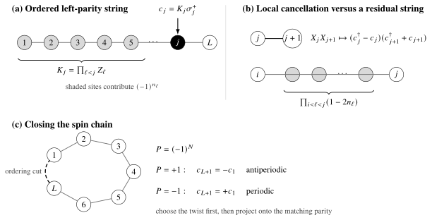
The operator at site $j$ carries the parity of every earlier occupation. Adjacent even products cancel their common strings, but separated operators retain the parity of intervening sites. Closing a periodic spin chain makes the boundary term depend on total fermion parity $P=(-1)^N$, so even and odd sectors use different fermionic twists.

Global Fermion Parity

The total fermion number is

$$N = \sum_{j=1}^{L}n_j.$$

Its parity is

$$P = (-1)^N = e^{i\pi N} = \prod_{j=1}^{L}(1-2n_j) = \prod_{j=1}^{L}Z_j.$$

An operator with an even number of $c$ and $c^\dagger$ factors commutes with $P$. An odd operator anticommutes with it. Number-nonconserving quadratic spin chains therefore often retain exact parity even when they do not retain exact fermion number.

For the rotated transverse-field Ising chain below, $P$ is exactly the global spin-flip symmetry of the original spin convention.

Open Chains

For an open chain, every nearest-neighbor bond lies inside the chosen order. No interaction closes from site $L$ back to site $1$, so no full-chain string appears.

The map is then a direct equality between the complete $2^L$-dimensional spin Hilbert space and the complete $2^L$-dimensional fermion Fock space. One may still block diagonalize by parity when the Hamiltonian preserves it, but no parity-dependent boundary condition is needed to define the transformed open Hamiltonian.

Open chains are therefore the cleanest setting for a first derivation. They also expose edge Majorana operators in the Ising example without the extra ring closure term.

Periodic Spin Chains

Suppose the spin Hamiltonian contains a boundary bond between sites $L$ and $1$. The local cancellation used for $j<L$ no longer applies in the same way because the chosen order has a cut between those sites.

For the transverse product,

$$X_LX_1 = -P \left(c_L^\dagger-c_L\right) \left(c_1^\dagger+c_1\right).$$

The minus sign follows from moving the total parity operator past one odd local fermion factor. Therefore a periodic spin coupling $-JX_LX_1$ becomes

$$+JP \left(c_L^\dagger-c_L\right) \left(c_1^\dagger+c_1\right).$$

The transformed Hamiltonian is still quadratic within a fixed parity sector, because $P$ can then be replaced by its eigenvalue $p=\pm1$. It is not one unrestricted quadratic Hamiltonian with one universal boundary condition.

Effective Fermion Boundary Condition

The bulk expression can be extended uniformly through the boundary by imposing

$$c_{L+1} = -p c_1.$$

Hence

Fixed parity	Effective fermion boundary	Allowed wave numbers
$p=+1$ (even $N$)	antiperiodic, $c_{L+1}=-c_1$	$k=(2m+1)\pi/(La)$
$p=-1$ (odd $N$)	periodic, $c_{L+1}=c_1$	$k=2\pi m/(La)$

This table uses the convention of this page and an untwisted periodic spin ring. A staggered gauge change can shift signs and momenta, but it cannot remove the need to correlate the fermion boundary with parity.

Projection Is Still Required

Fixing $p$ determines the boundary condition used to diagonalize the quadratic Hamiltonian. One must also retain only many-body states with the same physical parity:

$$(-1)^N = p.$$

Bogoliubov transformations preserve parity even though they mix particle and hole operators. Failing to impose the final sector projection can double the spin Hilbert space or select an unphysical candidate ground state.

The periodic momentum set may contain self-inverse modes $k=0$ and $k=\pi/a$. These occur in the periodic fermion sector when allowed by $L$ and must be treated separately from paired $k,-k$ blocks.

The Anisotropic XY Chain

Before specializing to Ising, consider

$$\begin{aligned} H_{XY} = {}& -J \sum_j \left[ \frac{1+\gamma}{2}X_jX_{j+1} + \frac{1-\gamma}{2}Y_jY_{j+1} \right] \\ &- h \sum_jZ_j. \end{aligned}$$

For an open chain, Jordan–Wigner gives

$$\begin{aligned} H_{XY} = {}& -J \sum_{j=1}^{L-1} \bigl[ c_j^\dagger c_{j+1} + c_{j+1}^\dagger c_j \\ &\qquad\qquad + \gamma \left( c_j^\dagger c_{j+1}^\dagger - c_jc_{j+1} \right) \bigr] \\ &- h \sum_{j=1}^{L} (1-2n_j). \end{aligned}$$

At $\gamma=0$, the pairing vanishes and total fermion number is conserved. At $\gamma\ne0$, only parity is conserved. At $\gamma=1$, the exchange is $-J\sum_jX_jX_{j+1}$, the rotated transverse-field Ising chain.

The map makes the distinction between integrability and number conservation explicit. A quadratic Bogoliubov Hamiltonian can be exactly solvable even when it creates and annihilates fermion pairs.

Transverse-Field Ising Example

Start from the convention used on the model page:

$$H_{\mathrm{TFIM}} = -J \sum_j \sigma_j^z\sigma_{j+1}^z - h \sum_j\sigma_j^x.$$

The $\sigma$ symbols here denote the original physical axes. Rotate the spin coordinates by defining

$$X_j = \sigma_j^z, \qquad Z_j = \sigma_j^x, \qquad Y_j = -\sigma_j^y.$$

These operators satisfy the same Pauli algebra, and

$$H_{\mathrm{TFIM}} = -J \sum_jX_jX_{j+1} - h \sum_jZ_j.$$

Open-Chain Fermion Hamiltonian

For an open chain,

$$\begin{aligned} H_{\mathrm O} = {}& -J \sum_{j=1}^{L-1} \left(c_j^\dagger-c_j\right) \left(c_{j+1}^\dagger+c_{j+1}\right) \\ &- h \sum_{j=1}^{L} (1-2n_j). \end{aligned}$$

Expanding the bond term gives

$$\begin{aligned} H_{\mathrm O} = {}& -J \sum_{j=1}^{L-1} \bigl( c_j^\dagger c_{j+1} + c_{j+1}^\dagger c_j \\ &\qquad\qquad + c_j^\dagger c_{j+1}^\dagger - c_jc_{j+1} \bigr) \\ &+ 2h \sum_{j=1}^{L}n_j - hL. \end{aligned}$$

This is quadratic but not number conserving. Its exact symmetry is

$$P = (-1)^N = \prod_jZ_j = \prod_j\sigma_j^x.$$

Thus the original global Ising spin flip becomes fermion parity.

Majorana Form

Define two Majorana operators per site,

$$a_j = c_j+c_j^\dagger, \qquad b_j = i(c_j^\dagger-c_j).$$

They obey

$$a_j^\dagger=a_j, \qquad b_j^\dagger=b_j,$$

and

$$\{a_i,a_j\} = \{b_i,b_j\} = 2\delta_{ij}, \qquad \{a_i,b_j\} = 0.$$

Since

$$Z_j = -ia_jb_j,$$

the open Hamiltonian becomes

$$H_{\mathrm O} = i h \sum_{j=1}^{L}a_jb_j + i J \sum_{j=1}^{L-1}b_ja_{j+1}.$$

The field couples the two Majoranas on the same site; exchange couples Majoranas across neighboring sites. At $J=0$, every site is paired internally. At $h=0$, $a_1$ and $b_L$ are absent from the Hamiltonian. The model-specific meaning of these limits and their finite-size splitting belongs to the transverse-field Ising and Kitaev-chain pages.

Periodic Chain and Fourier Transform

For a periodic spin ring, first choose $p=\pm1$ and impose

$$c_{L+1} = -p c_1.$$

Then use

$$c_j = \frac1{\sqrt L} \sum_k e^{ikja}c_k,$$

with the momentum grid appropriate to $p$. Pair $k$ with $-k$ and introduce

$$\Psi_k = \begin{pmatrix} c_k\\ c_{-k}^\dagger \end{pmatrix}.$$

Up to an additive constant and separate self-inverse modes, the Bogoliubov–de Gennes matrix may be written

$$\mathcal H(k) = 2 \left[ (h-J\cos ka)\tau_z + J\sin(ka)\tau_y \right].$$

Its eigenvalues are $\pm\varepsilon(k)$, where

$$\begin{aligned} \varepsilon(k) &= 2 \sqrt{ (h-J\cos ka)^2 + J^2\sin^2(ka) } \\ &= 2J \sqrt{ 1+g^2-2g\cos(ka) }, \end{aligned}$$

with

$$g = \frac hJ.$$

The Jordan–Wigner step produced a quadratic paired-fermion problem. Fourier and Bogoliubov transformations finish the diagonalization. The bulk gap, critical point, phase structure, and finite-size interpretation are developed canonically in Transverse-Field Ising Model.

XXZ Crosswalk

For the spin operators associated with the Pauli axes of this page, define

$$s_j^x=\frac{X_j}{2}, \qquad s_j^y=\frac{Y_j}{2}, \qquad s_j^z=\frac{Z_j}{2}.$$

In the primary occupation convention,

$$s_j^z = \frac12-n_j.$$

An open XXZ chain maps to

$$\begin{aligned} H_{\mathrm{XXZ}} = {}& \frac J2 \sum_{j=1}^{L-1} \left( c_j^\dagger c_{j+1} + c_{j+1}^\dagger c_j \right) \\ &+ J\Delta \sum_{j=1}^{L-1} \left(n_j-\frac12\right) \left(n_{j+1}-\frac12\right) \\ &+ h \sum_{j=1}^{L} \left(n_j-\frac12\right). \end{aligned}$$

After the spin-axis rotation used by the XXZ page, the final field term changes sign. The density interaction remains for $\Delta\ne0$, so Jordan–Wigner does not make the generic XXZ chain free. It changes a spin interaction into an interacting spinless-fermion Hamiltonian.

What the Transformation Does and Does Not Preserve

It preserves exactly:

• the finite-dimensional spectrum when boundaries and sectors are mapped correctly;
• matrix elements after every operator and state is transformed consistently;
• the Hilbert-space dimension;
• algebraic products and adjoints;
• global symmetries, though their expressions can change.

It does not generally preserve:

• geometric locality of odd or separated operators;
• ordinary particle number;
• a universal boundary condition independent of parity;
• manifest translation symmetry at the chosen ordering cut;
• free-particle structure for interacting spin models;
• locality under a naive higher-dimensional mode ordering.

Jordan–Wigner is also not a Bogoliubov transformation. A Bogoliubov transformation is linear in fermionic creation and annihilation operators. Jordan–Wigner is a nonlocal nonlinear dictionary between commuting spin-site algebras and a graded fermion algebra.

Computational Use

In qubit simulation, the direct encoding is

$$c_j = \frac12 \left( \prod_{\ell<j}Z_\ell \right) (X_j+iY_j).$$

A hopping term between modes $i<j$ becomes Pauli strings with $Z$ operators between the endpoints. Mode ordering therefore affects Pauli weight and circuit cost even though it does not change the target fermionic Hamiltonian.

For exact diagonalization, the same signs are often implemented directly in occupation bits:

$$\begin{aligned} q_j &= \operatorname{popcount} (\text{occupied modes left of }j), \\ \text{sign} &= (-1)^{q_j}. \end{aligned}$$

These are two implementations of the same parity rule. A reliable code test compares the resulting $c_j$ matrices against the canonical anticommutators and checks a few basis-state actions by hand.

Common Mistakes

• Omitting the parity string because local occupations already satisfy $n_j=0,1$.
• Switching between $n=(1-Z)/2$ and $n=(1+Z)/2$ without rotating the spin axes.
• Using a nearest-neighbor cancellation formula for separated sites.
• Calling every Jordan–Wigner image a free-fermion Hamiltonian.
• Forgetting that anisotropic $XY$ exchange creates and annihilates fermion pairs.
• Treating a periodic spin ring as one unrestricted periodic fermion problem.
• Choosing the even or odd boundary grid without projecting onto the matching parity sector.
• Pairing $k$ and $-k$ while overlooking self-inverse $k=0$ or $k=\pi/a$ modes.
• Imposing spin-derived parity boundaries on a fermion ring defined independently.
• Saying the map fails algebraically in higher dimensions when the actual generic failure is locality.
• Comparing local spin and local fermion correlators as though the operator map were local.
• Describing Jordan–Wigner as a linear canonical or Bogoliubov rotation.

Exercises

Exercise 1: Onsite algebra

Starting from $c_j=K_j\sigma_j^+$, prove $c_j^2=0$ and $\{c_j,c_j^\dagger\}=I$.

Solution

The string contains only sites to the left, so it commutes with $\sigma_j^\pm$. Since $K_j^2=I$,

$$c_j^2 = K_j^2(\sigma_j^+)^2 = 0.$$

Also,

$$\begin{aligned} \{c_j,c_j^\dagger\} &= K_j^2 \{\sigma_j^+,\sigma_j^-\} \\ &= I. \end{aligned}$$

The result uses only the one-site Pauli ladder algebra.

Exercise 2: Offsite minus sign

Let $i<j$. Show explicitly that $c_ic_j=-c_jc_i$ and identify the factor that supplies the sign.

Solution

Write

$$K_j = K_iZ_iR_{ij}, \qquad R_{ij} = \prod_{i<\ell<j}Z_\ell.$$

All factors commute except the $Z_i$ factor and the ladder on site $i$. Using

$$\sigma_i^+Z_i=-\sigma_i^+, \qquad Z_i\sigma_i^+=\sigma_i^+,$$

gives

$$c_ic_j = -\sigma_i^+R_{ij}\sigma_j^+,$$

and

$$c_jc_i = +\sigma_i^+R_{ij}\sigma_j^+.$$

Thus $c_ic_j=-c_jc_i$. The single factor $Z_i$ inside the later operator’s string supplies the sign.

Exercise 3: Nearest-neighbor exchange

Derive the image of $X_jX_{j+1}+Y_jY_{j+1}$ and explain why it conserves fermion number.

Solution

Use

$$X_jX_{j+1} = (c_j^\dagger-c_j) (c_{j+1}^\dagger+c_{j+1}),$$

and

$$Y_jY_{j+1} = -(c_j^\dagger+c_j) (c_{j+1}^\dagger-c_{j+1}).$$

Adding cancels the pair-creation and pair-annihilation terms:

$$X_jX_{j+1} + Y_jY_{j+1} = 2 \left( c_j^\dagger c_{j+1} + c_{j+1}^\dagger c_j \right).$$

Each surviving term contains one creation and one annihilation operator, so it commutes with $N=\sum_jn_j$.

Exercise 4: A separated spin correlator

Map $X_1X_4$ to fermions. Which sites appear in the residual string?

Solution

The general formula gives

$$X_1X_4 = (c_1^\dagger-c_1) (1-2n_2)(1-2n_3) (c_4^\dagger+c_4).$$

Sites two and three lie strictly between the endpoints and therefore remain in the parity string. There is no factor from site one because its endpoint parity factor has already been used to convert $c_1+c_1^\dagger$ into $c_1^\dagger-c_1$.

Exercise 5: Boundary parity

Starting from the periodic spin term $-JX_LX_1$, derive its fermionic boundary term and the effective boundary condition in a fixed parity sector.

Solution

The final-site string is

$$K_L = \prod_{\ell=1}^{L-1}Z_\ell = PZ_L.$$

Moving $P$ through one odd local fermion factor produces a minus sign. Therefore

$$X_LX_1 = -P (c_L^\dagger-c_L) (c_1^\dagger+c_1).$$

Multiplying by $-J$ gives

$$+JP (c_L^\dagger-c_L) (c_1^\dagger+c_1).$$

In a parity sector $P=p$, this equals the uniform bulk expression if

$$c_{L+1} = -p c_1.$$

Even parity is therefore antiperiodic and odd parity periodic in this convention.

Exercise 6: Momentum grids on eight sites

List the dimensionless momenta $ka$ for an eight-site ring in the even- and odd-parity sectors. Which sector contains self-inverse modes?

Solution

Even fermion parity uses antiperiodic boundaries:

$$ka = \frac{(2m+1)\pi}{8}, \qquad m=0,1,\ldots,7.$$

Equivalently, representatives in $(-\pi,\pi]$ are

$$ka \in \left\{ \pm\frac\pi8, \pm\frac{3\pi}{8}, \pm\frac{5\pi}{8}, \pm\frac{7\pi}{8} \right\}.$$

Odd parity uses periodic boundaries:

$$ka = \frac{2\pi m}{8}.$$

Representatives are

$$ka \in \left\{ 0, \pm\frac\pi4, \pm\frac\pi2, \pm\frac{3\pi}{4}, \pi \right\}.$$

The periodic sector contains the self-inverse modes $0$ and $\pi$.

Exercise 7: Ising dispersion

Diagonalize the $2\times2$ matrix

$$\mathcal H(k) = 2 \left[ (h-J\cos ka)\tau_z + J\sin(ka)\tau_y \right]$$

and recover the bulk quasiparticle dispersion.

Solution

The two Pauli matrices anticommute and square to the identity. Therefore

$$\mathcal H(k)^2 = 4 \left[ (h-J\cos ka)^2 + J^2\sin^2(ka) \right]I.$$

The eigenvalues are $\pm\varepsilon(k)$ with

$$\begin{aligned} \varepsilon(k) &= 2 \sqrt{ (h-J\cos ka)^2 + J^2\sin^2(ka) } \\ &= 2J \sqrt{ 1+g^2-2g\cos(ka) }. \end{aligned}$$

The gap closes at $g=1$ and $k=0$ in the thermodynamic limit. Boundary and parity determine whether $k=0$ itself belongs to a finite-size momentum grid.

Exercise 8: Ordering in two dimensions

Order a $3\times3$ square lattice row by row. Compare the Jordan–Wigner string length for a horizontal nearest-neighbor bond and a vertical nearest-neighbor bond.

Solution

Horizontal neighbors inside one row are consecutive in the ordering. Their common parity strings cancel, leaving a bounded local fermion operator.

Vertical neighbors in adjacent rows differ by three positions in the row-major order. Their transformed bilinear retains parity factors for the modes lying between them. On a square lattice of width $W$, a vertical bond generally spans order $W$ modes.

The map remains exact, but the Pauli or fermion representation of a geometrically local vertical bond becomes increasingly nonlocal as the width grows. A different snake ordering moves which bonds are long; it cannot make every two-dimensional nearest-neighbor bond consecutive simultaneously.

Key Takeaways

• The parity string $K_j=\prod_{\ell<j}Z_\ell$ converts commuting spin-site ladders into canonical fermions.
• The string reproduces the occupation-basis sign $(-1)^{\sum_{\ell<j}n_\ell}$.
• Density is local, nearest-neighbor even products often become local, and separated transverse operators retain strings.
• One dimension is special because geometric nearest neighbors can be consecutive in one total ordering.
• Periodic spin boundaries produce a boundary term containing total fermion parity.
• In this convention, even parity uses antiperiodic fermions and odd parity uses periodic fermions.
• The anisotropic XY and transverse-field Ising chains become quadratic paired-fermion models; XXZ remains interacting away from its free point.
• Jordan–Wigner is an exact nonlocal algebra dictionary, not a Bogoliubov rotation and not a guarantee of free dynamics.

Further Reading

• Fermionic Anticommutation Relations
• Fermionic Operators in Many-Body Models
• Spinless Fermion Chains
• Transverse-Field Ising Model
• XXZ Spin Chain
• XY Model
• Kitaev Chain
• Number Operators and Conserved Quantities

References

1. P. Jordan and E. Wigner, “Über das Paulische Äquivalenzverbot”, Zeitschrift für Physik 47, 631–651 (1928).
2. E. Lieb, T. Schultz, and D. Mattis, “Two Soluble Models of an Antiferromagnetic Chain”, Annals of Physics 16, 407–466 (1961).
3. T. D. Schultz, D. C. Mattis, and E. H. Lieb, “Two-Dimensional Ising Model as a Soluble Problem of Many Fermions”, Reviews of Modern Physics 36, 856–871 (1964).
4. P. Pfeuty, “The One-Dimensional Ising Model with a Transverse Field”, Annals of Physics 57, 79–90 (1970).
5. E. Barouch and B. M. McCoy, “Statistical Mechanics of the XY Model. II. Spin-Correlation Functions”, Physical Review A 3, 786–804 (1971).
6. E. Fradkin, “Jordan–Wigner Transformation for Quantum-Spin Systems in Two Dimensions and Fractional Statistics”, Physical Review Letters 63, 322–325 (1989).
7. S. Sachdev, Quantum Phase Transitions, 2nd ed., Cambridge University Press (2011).
8. F. Franchini, An Introduction to Integrable Techniques for One-Dimensional Quantum Systems, Springer (2017).
9. S. B. Bravyi and A. Yu. Kitaev, “Fermionic Quantum Computation”, Annals of Physics 298, 210–226 (2002).