XXZ Spin Chain

The spin-$1/2$ XXZ chain is the nearest-neighbor Heisenberg chain with different exchange strengths along the distinguished $z$ axis and in the transverse $xy$ plane. In a standard convention,

$$H = J \sum_j \left( s_j^x s_{j+1}^x + s_j^y s_{j+1}^y + \Delta s_j^z s_{j+1}^z \right) - h \sum_j s_j^z.$$

Here $J$ and $h$ have units of energy, the $s_j^\alpha$ are dimensionless spin-$1/2$ operators, and $\Delta$ is the dimensionless exchange anisotropy. This one parameter connects a free-fermion chain, a gapless interacting quantum liquid, the isotropic antiferromagnet, a gapped Néel phase, and a ferromagnet.

The model is unusually valuable because several descriptions meet without becoming interchangeable. It is a local spin Hamiltonian, an interacting spinless-fermion model after a Jordan–Wigner transformation, an integrable many-body system solved by factorized scattering, and a compact-boson field theory at low energy in its critical regime. Each description answers a different class of questions.

Canonical Scope

The XXZ Chain dossier is the convention-complete lookup record for the baseline phase map, exact fingerprints, observables, and finite-ring validation set. This teaching article owns the detailed fermion, Bethe, Luttinger, BKT, transport, and correlation developments.

The Spin-$1/2$ Chain dossier owns the umbrella XYZ-family record, spin-versus-Pauli normalization, generic symmetry conditions, and finite-chain audit. This page owns the XXZ specialization and its anisotropy-dependent physics.

This page is the canonical home for the spin-$1/2$ XXZ chain: Hamiltonian conventions, anisotropy, symmetries, the zero-field phase diagram, exact finite checks, the fermion map, Bethe-ansatz structure, and the Luttinger-liquid bridge.

The Heisenberg Chain dossier owns the compact isotropic spin-$1/2$ record and benchmark, while Heisenberg Model owns isotropic exchange on general lattices, arbitrary spin, spin waves, and broader quantum-magnetism context. The Transverse-Field Ising Model owns the noncommuting-field Ising chain and its $c=1/2$ critical point. Correlation Functions Overview owns the general definitions of connected correlators and structure factors.

Spinless Fermion Chains owns the fermionic $t$–$V$ Hamiltonian, free-chain solution, fermionic correlators, twist response, and density-language phase interpretation. This page states the fermion dictionary only far enough to expose that connection; Jordan–Wigner Transformation owns the full derivation of nonlocal strings, periodic-boundary parity sectors, and operator dictionaries. Likewise, the Bethe ansatz is developed far enough to show what integrability means, but not as a substitute for a full exact-solutions treatment.

Degrees of Freedom and Units

For $L$ sites,

$$\mathcal H = \bigotimes_{j=1}^{L} \mathbb C^2, \qquad \dim\mathcal H = 2^L.$$

The dimensionless spin operators obey

$$\begin{aligned} [s_i^\alpha,s_j^\beta] &= i\delta_{ij} \epsilon_{\alpha\beta\gamma} s_j^\gamma, \\ \mathbf s_j^2 &= \frac34. \end{aligned}$$

Physical angular momentum is $\mathbf S_j=\hbar\mathbf s_j$. For spin $1/2$,

$$s_j^\alpha = \frac12\sigma_j^\alpha.$$

Therefore the same Hamiltonian in Pauli-matrix notation is

$$\begin{aligned} H = {}& \frac{J}{4} \sum_j \left( \sigma_j^x\sigma_{j+1}^x + \sigma_j^y\sigma_{j+1}^y + \Delta \sigma_j^z\sigma_{j+1}^z \right) \\ &- \frac{h}{2} \sum_j\sigma_j^z. \end{aligned}$$

Missing factors of two or four often come from comparing these two conventions. A quoted critical field, velocity, or energy density is not portable until the operator normalization is stated.

Open and Periodic Chains

For an open chain,

$$H_{\mathrm{OBC}} = J \sum_{j=1}^{L-1} \left( s_j^x s_{j+1}^x + s_j^y s_{j+1}^y + \Delta s_j^z s_{j+1}^z \right) - h\sum_{j=1}^{L}s_j^z.$$

For a periodic chain,

$$s_{L+1}^\alpha = s_1^\alpha,$$

and the exchange sum has $L$ bonds. Open chains have $L-1$ bonds. This difference is order one in the total energy but vanishes in the bulk energy density as $L\to\infty$.

Periodic spin boundary conditions do not become one universal periodic boundary condition for Jordan–Wigner fermions. The fermion boundary term depends on total fermion parity. Ignoring that sector dependence can shift finite-size momenta and apparent gaps.

Exchange Anisotropy

Write the exchange tensor as

$$J_x=J_y=J, \qquad J_z=J\Delta.$$

The parameter $\Delta$ compares longitudinal and transverse exchange:

Regime	Conventional name	Dominant tendency for $J>0$
$\Delta=0$	XX limit	transverse exchange and spin transport
$\lvert\Delta\rvert<1$	easy plane	fluctuating $xy$ correlations
$\Delta=1$	isotropic Heisenberg point	full rotationally invariant exchange
$\Delta>1$	antiferromagnetic easy axis	alternating $z$ alignment
$\Delta<-1$	ferromagnetic easy axis	uniform $z$ polarization

The phrases easy plane and easy axis describe the exchange anisotropy, not a proof that a finite one-dimensional ground state has a classical orientation. Quantum fluctuations, symmetry, and the thermodynamic limit still determine the phase.

Raising and Lowering Form

Define

$$s_j^\pm = s_j^x \pm i s_j^y.$$

Then

$$s_j^x s_{j+1}^x + s_j^y s_{j+1}^y = \frac12 \left( s_j^+s_{j+1}^- + s_j^-s_{j+1}^+ \right).$$

The Hamiltonian becomes

$$\begin{aligned} H = {}& \frac{J}{2} \sum_j \left( s_j^+s_{j+1}^- + s_j^-s_{j+1}^+ \right) \\ &+ J\Delta \sum_j s_j^z s_{j+1}^z - h\sum_j s_j^z. \end{aligned}$$

The transverse term moves a down spin relative to an up-spin background. The longitudinal term assigns an interaction energy according to neighboring $z$ projections. This separation anticipates the hopping-plus-density-interaction fermion form.

Continuous Spin Symmetry

For generic $\Delta$, simultaneous rotations of every spin about the $z$ axis leave the Hamiltonian invariant. The generator is

$$S_{\mathrm{tot}}^z = \sum_{j=1}^{L}s_j^z.$$

Because every transverse exchange term raises one site and lowers its neighbor,

$$[H,S_{\mathrm{tot}}^z] = 0.$$

The Hilbert space decomposes into fixed-magnetization sectors. If $M$ sites are down relative to the all-up state, then

$$S_{\mathrm{tot}}^z = \frac{L}{2}-M,$$

and the sector dimension is

$$\dim\mathcal H_M = \binom{L}{M}.$$

This $U(1)$ symmetry is both physical and computational: exact diagonalization can work one magnetization block at a time.

Symmetry Enhancement at the Isotropic Point

At $\Delta=1$ and $h=0$,

$$H = J\sum_j \mathbf s_j\cdot\mathbf s_{j+1},$$

so all components of total spin commute with $H$:

$$[H,S_{\mathrm{tot}}^\alpha] = 0, \qquad \alpha=x,y,z.$$

The internal symmetry is enhanced from axial $U(1)$ to $SU(2)$. A longitudinal field retains rotations about $z$ but lifts degeneracies between different values of $S_{\mathrm{tot}}^z$.

The SU(2) reference develops the group structure. The XXZ page uses only the consequence that $\Delta=1$ is a symmetry-enhanced point, not a generic representative of the entire anisotropic family.

Discrete and Lattice Symmetries

At $h=0$, a global $\pi$ rotation about the $x$ axis sends

$$s_j^z \longmapsto -s_j^z, \qquad s_j^y \longmapsto -s_j^y,$$

while leaving $s_j^x$ unchanged. It reverses the total magnetization and preserves the Hamiltonian.

For uniform periodic couplings, the model also has lattice translation and spatial inversion symmetry. At $h=0$ it is time-reversal invariant. Boundaries, bond alternation, disorder, Dzyaloshinskii–Moriya exchange, or site-dependent fields can remove some of these symmetries even if $S_{\mathrm{tot}}^z$ remains conserved.

Special Parameter Values

Several values of $\Delta$ organize the model:

Value	Structure
$\Delta=0$	XX chain; free spinless fermions after Jordan–Wigner
$\Delta=1$	antiferromagnetic isotropic Heisenberg chain; $SU(2)$ symmetry
$\Delta=-1$	singular ferromagnetic endpoint after a staggered rotation
$-1<\Delta<1$	gapless interacting Luttinger liquid
$\Delta>1$	gapped antiferromagnetic easy-axis regime
$\Delta<-1$	gapped ferromagnetic regime at zero field

The points $\Delta=-1$ and $\Delta=1$ are not equivalent endpoints. The former is a first-order boundary with quadratic low-energy dispersion at the endpoint. The latter is a Berezinskii–Kosterlitz–Thouless boundary at which a gap opens nonanalytically into the Néel phase.

Zero-Field Phase Diagram

Assume $J>0$, $h=0$, short-range nearest-neighbor exchange, and the thermodynamic limit.

Anisotropy	Ground-state regime	Gap	Long-distance structure
$\Delta<-1$	$z$-ferromagnet	gapped away from $\Delta=-1$	saturated magnetization
$-1<\Delta<1$	critical easy-plane phase	gapless	algebraic correlations, $c=1$
$\Delta=1$	isotropic critical point	gapless	algebraic correlations with logarithmic corrections
$\Delta>1$	easy-axis antiferromagnet	gapped	thermodynamic Néel order

The critical interval is a phase, not one isolated critical point. Its exponents vary continuously with $\Delta$ through the Luttinger parameter $K$.

Finite chains require more careful language. A finite even periodic chain in the critical or antiferromagnetic regimes may have a unique symmetry eigenstate. Thermodynamic order is diagnosed through size scaling, long-distance correlations, symmetry-partner structure, or a symmetry-breaking source with an explicit order of limits.

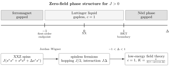
For $J>0$ and $h=0$, the spin-$1/2$ XXZ chain passes from a ferromagnet through a gapless $c=1$ phase into a gapped Néel phase. Jordan–Wigner maps the lattice model to spinless hopping with nearest-neighbor interaction, while the critical interval has a Luttinger-liquid description with an exactly known $K$.

Ferromagnetic Regime

For $\Delta<-1$, the all-up and all-down product states minimize the zero-field bulk energy. For a periodic chain,

$$\lvert F_\uparrow\rangle = \lvert\uparrow\uparrow\cdots\uparrow\rangle, \qquad \lvert F_\downarrow\rangle = \lvert\downarrow\downarrow\cdots\downarrow\rangle.$$

Their exchange energy is

$$E_F = \frac{J\Delta L}{4}.$$

The transverse exchange annihilates each fully polarized state. A single overturned spin can propagate, but at $h=0$ its minimum excitation energy is

$$\Delta_{\mathrm{mag}} = J(-\Delta-1), \qquad \Delta<-1.$$

This gap closes as $\Delta\to-1^-$.

The Endpoint at Minus One

On an even bipartite chain, rotate every other spin by $\pi$ about the $z$ axis. The transformation changes the signs of $s^x$ and $s^y$ on one endpoint of every bond while leaving $s^z$ unchanged. At $\Delta=-1$,

$$H(-1) \longmapsto -J \sum_j \mathbf s_j\cdot\mathbf s_{j+1}.$$

Thus the endpoint is unitarily equivalent to an isotropic ferromagnetic Heisenberg chain. Its finite-size ground space is much more degenerate than the generic critical ground state.

For spin $1/2$, the ferromagnetic total-spin multiplet has

$$S_{\mathrm{tot}} = \frac{L}{2}, \qquad \dim\mathcal G = 2S_{\mathrm{tot}}+1 = L+1.$$

The staggered rotation preserves this dimension at $\Delta=-1$ for the even bipartite chain.

The low-energy one-magnon dispersion near its minimum is quadratic, not relativistic. If $k=\pi+q$ at $h=0$,

$$\varepsilon(\pi+q) = J\left[1-\cos q\right] \sim \frac{Jq^2}{2}.$$

Consequently $\Delta=-1$ is not included as an ordinary $c=1$ conformal point of the interval $-1<\Delta<1$. Both the Luttinger velocity and the assumptions behind the linear low-energy theory become singular there.

Critical Easy-Plane Regime

For

$$-1 < \Delta < 1,$$

the chain is gapless. It has no conventional long-range transverse order, but spin correlations decay algebraically. Low-energy excitations live near two Fermi points in the fermion description and become collective density and phase modes once interactions are included.

This phase is a Luttinger liquid. Luttinger Liquid Preview owns the generic bosonization convention, vertex dimensions, and perturbation criteria; this page supplies the exact XXZ parameters and spin-operator realization. The phase has:

• linear low-energy dispersion;
• central charge $c=1$;
• continuously varying correlation exponents;
• power-law finite-size gaps of order $1/L$;
• logarithmic interval entanglement;
• no stable one-particle quasiparticle pole of an ordinary Fermi liquid.

The word liquid here names a universality class of one-dimensional gapless systems. It does not imply a continuum fluid at the microscopic scale.

The Isotropic Antiferromagnet

At $\Delta=1$, the spin-$1/2$ antiferromagnetic Heisenberg chain remains gapless. Its low-energy velocity is

$$v = \frac{\pi J a}{2\hbar},$$

where $a$ is the lattice spacing.

The continuum fixed point has $c=1$ and the limiting Luttinger value $K=1/2$ in the convention used below. A marginally irrelevant operator produces multiplicative logarithmic corrections. Finite-size fits that ignore those corrections can converge slowly and imitate shifted exponents.

The exact ground-state energy density is

$$\frac{e_0}{J} = \frac14 - \ln2.$$

This number is a useful normalization and numerical benchmark.

Antiferromagnetic Easy-Axis Regime

For $\Delta>1$, longitudinal exchange favors the two alternating configurations

$$\lvert N_1\rangle = \lvert\uparrow\downarrow\uparrow\downarrow\cdots\rangle,$$

and

$$\lvert N_2\rangle = \lvert\downarrow\uparrow\downarrow\uparrow\cdots\rangle.$$

At large $\Delta$, the transverse exchange creates quantum fluctuations around these Ising-like configurations. The thermodynamic phase has staggered $z$ order and a nonzero bulk gap.

A convenient order parameter is the staggered magnetization

$$m_{\mathrm{st}} = \lim_{L\to\infty} \frac1L \sum_{j=1}^{L} (-1)^j \langle s_j^z\rangle,$$

with a symmetry-breaking prescription understood. In a finite translation-invariant state, $\langle s_j^z\rangle$ may vanish even when

$$\lim_{r\to\infty} (-1)^r \langle s_j^z s_{j+r}^z\rangle \ne 0$$

after the thermodynamic limit.

The Transition at One

The boundary at $\Delta=1$ is of Berezinskii–Kosterlitz–Thouless type. The critical side approaches $K=1/2$, while an umklapp perturbation becomes relevant on the easy-axis side and pins the low-energy field.

The gap does not open as a simple power

$$\Delta_{\mathrm{gap}} \not\propto (\Delta-1)^\nu$$

with an ordinary finite exponent $\nu$. It has an essential singularity. This makes numerical location of the transition delicate: modest sizes can remain much shorter than the rapidly growing correlation length.

Quantum Phase Transitions owns the general scaling language, while Renormalization Group Preview owns fixed lines, marginal directions, and BKT-type flow geometry. Here the important model-specific fact is that the first-order boundary at $\Delta=-1$ and the BKT boundary at $\Delta=1$ require different diagnostics.

A One-Magnon Check

Let

$$\lvert F_\uparrow\rangle = \lvert\uparrow\uparrow\cdots\uparrow\rangle$$

and define a one-down-spin basis

$$\lvert j\rangle = s_j^- \lvert F_\uparrow\rangle.$$

For a periodic chain, the polarized-state energy is

$$E_F = \frac{J\Delta L}{4} - \frac{hL}{2}.$$

Acting on $\lvert j\rangle$ gives

$$\begin{aligned} (H-E_F)\lvert j\rangle = {}& (h-J\Delta)\lvert j\rangle \\ &+ \frac{J}{2} \left( \lvert j-1\rangle + \lvert j+1\rangle \right). \end{aligned}$$

The momentum state

$$\lvert k\rangle = \frac1{\sqrt L} \sum_{j=1}^{L} e^{ikj}\lvert j\rangle$$

has excitation energy

$$\varepsilon(k) = h - J\Delta + J\cos k.$$

For $J>0$, the minimum is at $k=\pi$. The all-up state is stable when

$$h \ge h_{\mathrm{sat}} = J(1+\Delta).$$

For $\Delta>-1$, this is the positive saturation field in the stated convention. For $\Delta<-1$, the zero-field chain is already ferromagnetic.

Exact Two-Site Spectrum

Consider one open bond at $h=0$,

$$H_2 = J \left( s_1^x s_2^x + s_1^y s_2^y + \Delta s_1^z s_2^z \right).$$

The parallel states have energies

$$E_{\uparrow\uparrow} = E_{\downarrow\downarrow} = \frac{J\Delta}{4}.$$

In the zero-magnetization sector, define

$$\lvert t_0\rangle = \frac{ \lvert\uparrow\downarrow\rangle + \lvert\downarrow\uparrow\rangle }{\sqrt2}$$

and

$$\lvert s\rangle = \frac{ \lvert\uparrow\downarrow\rangle - \lvert\downarrow\uparrow\rangle }{\sqrt2}.$$

Their energies are

$$E_{t_0} = \frac{J(2-\Delta)}{4}, \qquad E_s = -\frac{J(2+\Delta)}{4}.$$

At $\Delta=1$, the three triplet states become degenerate at $J/4$, while the singlet lies at $-3J/4$. At $\Delta=-1$, the parallel states cross the singlet. This dimer detects the ferromagnetic boundary, but it cannot reproduce the thermodynamic distinction between a Luttinger liquid and a Néel phase.

Jordan–Wigner Dictionary

Introduce spinless fermions satisfying

$$\{c_i,c_j^\dagger\} = \delta_{ij}, \qquad \{c_i,c_j\} = 0.$$

One useful convention is

$$s_j^z = n_j - \frac12, \qquad n_j = c_j^\dagger c_j,$$

and

$$s_j^+ = c_j^\dagger \exp\!\left( i\pi \sum_{\ell<j}n_\ell \right).$$

The nonlocal string makes spin operators on different sites commute while the $c_j$ anticommute. For adjacent sites, the strings cancel locally in the exchange term.

For an open chain,

$$\begin{aligned} H = {}& \frac{J}{2} \sum_{j=1}^{L-1} \left( c_j^\dagger c_{j+1} + c_{j+1}^\dagger c_j \right) \\ &+ J\Delta \sum_{j=1}^{L-1} \left(n_j-\frac12\right) \left(n_{j+1}-\frac12\right) \\ &- h \sum_{j=1}^{L} \left(n_j-\frac12\right). \end{aligned}$$

Thus

$$t = \frac{J}{2}, \qquad V = J\Delta,$$

up to a removable sign of $t$ from a staggered fermion phase convention. The XXZ chain is the nearest-neighbor interacting spinless-fermion chain at a filling fixed by magnetization.

What the Fermion Map Explains

The dictionary makes several facts immediate:

• total magnetization becomes total fermion number, up to a constant;
• transverse exchange becomes nearest-neighbor hopping;
• longitudinal exchange becomes a nearest-neighbor density interaction;
• the field becomes a chemical-potential term;
• $\Delta=0$ is free;
• $\Delta\ne0$ is interacting even though the spin Hamiltonian remains integrable;
• the zero-field spin-flip symmetry fixes half filling in the nonmagnetic ground state.

It also shows what Jordan–Wigner does not accomplish. For $\Delta\ne0$, the density interaction remains. The map changes variables; it does not by itself diagonalize the model.

Free-Fermion XX Limit

At $\Delta=0$, the interaction vanishes. After a staggered gauge transformation if desired, the dispersion can be written

$$\epsilon(k) = -J\cos k - h.$$

At $h=0$, the ground state is half filled, with Fermi points

$$k_F = \pm\frac{\pi}{2}.$$

The energy density is

$$e_0 = -\frac{J}{\pi},$$

and the Fermi velocity is

$$v_F = \frac{Ja}{\hbar}.$$

The free point already has algebraic spin correlations because spin-flip operators contain Jordan–Wigner strings. A free fermion Hamiltonian does not imply that every spin observable is a one-body fermion observable.

Why the Interacting Chain Is Integrable

The uniform nearest-neighbor XXZ chain belongs to a family generated by the six-vertex transfer matrix. The Yang–Baxter relation implies commuting transfer matrices,

$$[T(u),T(v)] = 0,$$

for spectral parameters $u$ and $v$. Expanding a logarithm of $T(u)$ generates mutually commuting conserved quantities. The Hamiltonian is one member of that hierarchy.

This algebraic statement is stronger than energy conservation and total-magnetization conservation. It constrains many-body scattering so that it factorizes into compatible two-body processes.

Integrability is fragile under generic perturbations. Next-nearest-neighbor exchange, generic disorder, transverse fields, or arbitrary staggered couplings usually destroy the commuting hierarchy even when some ordinary symmetries survive.

The interacting random-field problem and the evidence required to distinguish localization from slow finite-time dynamics are treated in Many-Body Localization Preview.

Coordinate Bethe Ansatz

Choose the all-up state as a reference and work in a sector with $M$ down spins at ordered positions

$$1 \le x_1 < x_2 < \cdots < x_M \le L.$$

Away from collisions, the wavefunction is a superposition of plane waves:

$$\psi(x_1,\ldots,x_M) = \sum_{P\in S_M} A(P) \exp\!\left( i\sum_{a=1}^{M} k_{P_a}x_a \right).$$

The amplitudes for permutations are related by two-body scattering phases. Periodicity requires each quasiparticle to accumulate both its free phase around the ring and its scattering phases through every other quasiparticle. Schematically,

$$e^{ik_jL} = \prod_{\ell\ne j} S(k_j,k_\ell).$$

These coupled quantization conditions are the Bethe equations. The energy remains additive in the Bethe momenta,

$$E = E_F + \sum_{j=1}^{M} \left( h - J\Delta + J\cos k_j \right),$$

but the allowed $k_j$ are strongly correlated by the scattering equations.

A Rapidity Form of the Bethe Equations

In the critical regime, parameterize

$$\Delta = \cos\gamma, \qquad 0<\gamma<\pi.$$

A representative rapidity convention uses

$$e^{ik(\lambda)} = \frac{ \sinh(\lambda+i\gamma/2) }{ \sinh(\lambda-i\gamma/2) }.$$

The periodic Bethe equations then take the form

$$\left[ \frac{ \sinh(\lambda_j+i\gamma/2) }{ \sinh(\lambda_j-i\gamma/2) } \right]^L = \prod_{\ell\ne j} \frac{ \sinh(\lambda_j-\lambda_\ell+i\gamma) }{ \sinh(\lambda_j-\lambda_\ell-i\gamma) }.$$

Different sources shift, rescale, or negate rapidities and may include an overall phase in the equations. Those forms can be equivalent. A convention must be checked by reconstructing momentum, energy, and the one-magnon limit.

What Exact Solvability Does and Does Not Give

The Bethe equations determine finite-volume eigenvalues and eigenstates in principle. In practice:

• the number of roots grows with system size;
• roots can form complex patterns associated with bound states;
• selecting the ground-state root distribution requires care;
• finite-temperature thermodynamics leads to coupled nonlinear integral equations;
• norms and matrix elements require determinant formulas;
• dynamical correlation functions need sums over many intermediate states;
• special anisotropies can carry additional degeneracies and root subtleties.

“Exactly solvable” therefore does not mean “every observable has an elementary closed form.” It means that a nonperturbative spectral structure is available and can anchor controlled analytic and numerical work.

Thermodynamic Bethe Ansatz Preview

As $L,M\to\infty$ at fixed density, discrete Bethe roots condense into distributions. Sums become integrals,

$$\frac1L \sum_{j=1}^{M} f(\lambda_j) \longrightarrow \int d\lambda\, \rho(\lambda)f(\lambda).$$

The logarithmic Bethe equations become integral equations for root and hole densities. At finite temperature, minimizing the free energy subject to those constraints produces thermodynamic Bethe-ansatz equations for dressed energies.

This procedure is model-specific. Ordinary canonical and grand-canonical ensembles remain the statistical framework; integrability supplies an exact way to evaluate their thermodynamics for this special Hamiltonian. Post-quench stationary root densities and the charge-completeness problem are developed in Integrability and Generalized Gibbs Ensembles Preview.

Exact Bulk Benchmarks

Three zero-field results are especially useful for checking code and conventions:

Point	Exact bulk result
$\Delta=0$	$e_0/J=-1/\pi$
$\Delta=1$	$e_0/J=1/4-\ln2$
$\Delta<-1$ polarized branch	$e_F/J=\Delta/4$

The values assume the unshifted spin-operator Hamiltonian written at the top of this page. Adding a bond constant such as $-J\Delta/4$ changes every quoted energy density but not eigenstates, gaps, or phase boundaries.

Luttinger-Liquid Hamiltonian

Throughout $-1<\Delta<1$, the long-wavelength sector is described by conjugate compact fields $\phi(x)$ and $\theta(x)$. One common normalization is

$$[\phi(x),\partial_y\theta(y)] = i\pi\delta(x-y).$$

The universal quadratic Hamiltonian is

$$H_{\mathrm{LL}} = \frac{\hbar v}{2\pi} \int dx \left[ K(\partial_x\theta)^2 + \frac1K(\partial_x\phi)^2 \right].$$

The velocity $v$ sets the low-energy light cone. The dimensionless Luttinger parameter $K$ sets scaling dimensions and the relative stiffness of density and phase fluctuations.

The numerical value called $K$ depends on field normalization. Formulas must be compared as a complete package: commutator, Hamiltonian, operator dictionary, and correlation exponents.

Exact Luttinger Parameters at Zero Magnetization

For

$$\Delta = \cos\gamma, \qquad 0<\gamma<\pi,$$

the zero-field XXZ chain has

$$K = \frac{\pi}{2(\pi-\gamma)}$$

and

$$v = \frac{Ja}{\hbar} \frac{\pi\sin\gamma}{2\gamma}.$$

Useful checks are

$$\begin{array}{c|c|c} \Delta & K & v \\ \hline 0 & 1 & Ja/\hbar \\ 1^- & 1/2 & \pi Ja/(2\hbar) \\ -1^+ & \infty & 0 \end{array}$$

The divergent $K$ and vanishing $v$ at $\Delta\to-1^+$ signal the failure of an ordinary finite-velocity conformal description at the endpoint.

Long-Distance Correlations

At zero magnetization and away from endpoint subtleties, the leading forms are

$$\begin{aligned} \langle s_0^z s_r^z\rangle \sim {}& -\frac{K}{2\pi^2r^2} + A_z \frac{(-1)^r}{r^{2K}}, \\ \langle s_0^+s_r^-\rangle \sim {}& A_\perp \frac{(-1)^r}{r^{1/(2K)}}. \end{aligned}$$

The amplitudes $A_z$ and $A_\perp$ are nonuniversal. The exponents are universal once the $K$ convention is fixed.

At the XX point, $K=1$, so the leading transverse exponent is $1/2$. At the isotropic limit, $K=1/2$, and the leading staggered longitudinal and transverse powers both approach $1/r$, as required by restored spin rotation symmetry. Multiplicative logarithms modify the pure powers at $\Delta=1$.

Correlation Does Not Mean Order

An algebraic correlator tends to zero as $r\to\infty$. The gapless phase therefore has quasi-long-range order rather than a nonzero transverse order parameter. By contrast, in the easy-axis Néel phase,

$$(-1)^r \langle s_0^z s_r^z\rangle \longrightarrow m_{\mathrm{st}}^2$$

in an appropriate thermodynamic state.

Distinguishing these behaviors requires distance and size scaling. A large short-distance staggered correlator on one small chain is not enough.

Entanglement and Central Charge

For a periodic critical chain of physical circumference $\mathcal L=La$, the ground-state entropy of an interval of length $\ell$ is

$$S(\ell) = \frac{c}{3} \ln\!\left[ \frac{\mathcal L}{\pi a_0} \sin\!\left( \frac{\pi\ell}{\mathcal L} \right) \right] + s_1 + \cdots.$$

Here $a_0$ is a short-distance cutoff, $s_1$ is nonuniversal, and

$$c = 1$$

throughout the Luttinger-liquid regime. Open chains have the leading coefficient $c/6$ for an interval adjacent to a boundary.

In either gapped phase, interval entanglement saturates once $\ell$ greatly exceeds the correlation length, apart from finite cat-state or boundary contributions. Entanglement Entropy in Many-Body Systems owns the general scaling theory and numerical caveats.

Finite-Size Conformal Spectrum

For a periodic critical chain,

$$E_0(L) = Le_\infty - \frac{\pi\hbar v c}{6La} + o(L^{-1}).$$

Low-energy gaps behave as

$$E_n(L)-E_0(L) = \frac{2\pi\hbar v}{La} x_n + o(L^{-1}),$$

where $x_n$ are scaling dimensions, with momentum and winding quantum numbers determined by the compact boson.

These formulas provide a numerical route to $v$, $c$, and $K$, but subleading corrections matter. Near $\Delta=1$, marginal logarithms make naive straight-line extrapolations unreliable.

Spin Current

Conservation of $S_{\mathrm{tot}}^z$ implies a lattice continuity equation. With

$$\dot s_j^z = \mathcal J_{j-1}^z - \mathcal J_j^z,$$

one convention for the physical current is

$$\mathcal J_j^z = \frac{J}{\hbar} \left( s_j^x s_{j+1}^y - s_j^y s_{j+1}^x \right).$$

The anisotropy term does not move $z$ magnetization; the transverse exchange does. Transport in integrable chains is subtle because conserved quantities can protect ballistic components in some regimes and ensembles. A transport claim must specify temperature, field, order of limits, and the measured response. Transport Coefficients Preview supplies the generic Drude-weight, diffusion, Green–Kubo, and finite-size dictionary; this page retains the model-specific current.

Longitudinal Field

The field $h$ is conjugate to total magnetization. In the fermion language it is a chemical potential. It changes the filling and therefore changes the Luttinger parameter away from the zero-magnetization formula quoted above.

For $-1<\Delta\le1$, a finite interval below saturation remains a gapless Luttinger liquid. At

$$|h| = h_{\mathrm{sat}} = J(1+\Delta),$$

the ground state becomes fully polarized in the stated convention.

For $\Delta>1$, the zero-field Néel phase survives up to a lower critical field set by its gap. Between that field and saturation lies a field-induced gapless regime. The exact lower critical field and dressed parameters require Bethe-ansatz thermodynamics; they are not given by the one-magnon saturation calculation.

Finite Temperature

The zero-field phases above describe $T=0$. A one-dimensional short-range chain has no nonzero-temperature transition into true ferromagnetic or Néel long-range order. Thermal domain walls give a finite correlation length for every $T>0$.

Low-temperature observables can nevertheless retain quantum-critical scaling over large windows when

$$k_BT \ll J$$

and other gaps or crossover scales are controlled. Calling such a window a phase transition would conflate a crossover with the zero-temperature phase boundary.

Boundary Conditions and Parity

Three boundary issues should be kept separate:

1. Open and periodic spin chains have different bond counts and finite-size spectra.
2. Jordan–Wigner turns a periodic spin boundary into a fermion boundary term containing total parity.
3. Bethe equations depend on periodicity, twists, magnetization sector, and rapidity convention.

For bulk thermodynamics these differences often become subextensive. For exact spectra, momentum quantum numbers, entanglement cuts, and edge physics they remain essential.

A twist can be introduced by

$$s_{L+1}^\pm = e^{\pm i\Phi} s_1^\pm.$$

The dependence of the ground-state energy on $\Phi$ probes spin stiffness. The normalization of stiffness or Drude weight must be stated because conventions differ by factors of $L$, $\pi$, and $\hbar$.

Numerical Representation

In the $s^z$ product basis, the longitudinal exchange and field are diagonal. Each transverse bond either annihilates a parallel pair or exchanges

$$\lvert\uparrow\downarrow\rangle \longleftrightarrow \lvert\downarrow\uparrow\rangle.$$

The Hamiltonian is sparse. Within a fixed-$M$ sector, a basis state connects to at most the number of domain walls that can be exchanged across neighboring bonds.

Useful methods include:

• exact diagonalization in fixed magnetization and momentum sectors;
• Lanczos or Krylov methods for low energies and dynamics;
• matrix-product states and density-matrix renormalization for open chains;
• Bethe-root solvers for integrable finite systems;
• thermodynamic Bethe ansatz for bulk finite-temperature quantities;
• quantum Monte Carlo in sign-compatible formulations;
• conformal finite-size and entanglement fits in the critical regime.

Sparse Matrices explains the storage logic shared by local lattice Hamiltonians.

Diagnostics by Regime

Question	Useful diagnostic	Main caveat
ferromagnetic order	$S_{\mathrm{tot}}^z$, polarization, one-magnon gap	finite symmetry sectors and field selection
Luttinger liquid	$1/L$ gaps, algebraic correlations, $c=1$ entropy	logarithmic and boundary corrections
Néel order	staggered structure factor and long-distance $zz$ correlations	finite symmetric states can have zero one-point order
BKT boundary	level spectroscopy, stiffness, correlation exponents	exponentially large crossover length
integrability	level statistics, conserved charges, Bethe benchmarks	ordinary symmetries alone do not prove integrability
fermion mapping	spectra and fixed-number blocks	periodic parity sectors and string observables

No one scalar diagnostic identifies every phase and transition reliably.

Model Variants

Common extensions include:

• bond-alternating or dimerized XXZ chains;
• next-nearest-neighbor and frustrated exchange;
• random fields or random bonds;
• long-range exchange;
• Dzyaloshinskii–Moriya interactions;
• open chains with boundary fields or impurities;
• higher-spin anisotropic chains;
• ladders and coupled chains;
• quenches and periodic driving.

Some variants retain integrability for special boundary or coupling choices, but generic extensions do not. Phase diagrams and low-energy theories must be re-established rather than inherited automatically from the uniform nearest-neighbor chain.

Common Mistakes

• Omitting whether $s^\alpha$ or $\sigma^\alpha$ appears in the Hamiltonian.
• Calling every $|\Delta|<1$ point “the XX model”; only $\Delta=0$ is free.
• Saying Jordan–Wigner solves the interacting chain without mentioning the remaining density interaction.
• Treating $\Delta=-1$ as an ordinary relativistic $c=1$ endpoint.
• Treating the transition at $\Delta=1$ as a conventional power-law critical point.
• Inferring Néel order from a nonzero finite-distance correlator on one small chain.
• Inferring absence of order from a vanishing finite-system one-point function.
• Comparing $K$ values from incompatible bosonization normalizations.
• Using the zero-magnetization formulas for $K$ and $v$ at finite field.
• Forgetting logarithmic corrections at the isotropic point.
• Imposing periodic fermion boundary conditions without checking parity.
• Assuming integrability makes dynamical correlators elementary.
• Quoting a saturation field without the Hamiltonian and spin normalization.
• Confusing a low-temperature quantum-critical crossover with a finite-temperature phase transition.

Practical Reading Workflow

For an XXZ calculation:

1. Write the Hamiltonian and operator normalization.
2. State $J$, $\Delta$, $h$, $L$, and boundary conditions.
3. Identify exact symmetries and the magnetization sector.
4. Decide whether the target is a finite spectrum, bulk phase, correlator, or response.
5. Use a soluble limit: dimer, one magnon, $\Delta=0$, or $\Delta=1$.
6. If using Jordan–Wigner, record the $s^z$ convention and boundary parity.
7. If using Bethe ansatz, record the rapidity and energy convention.
8. If using Luttinger theory, record the field normalization, $K$, $v$, and validity window.
9. Scale in size, distance, or temperature before assigning a phase.
10. Separate exact statements from numerical extrapolation and low-energy approximation.

Cross-Links

• Many-Body and Quantum Statistical Mechanics
• XXZ Chain dossier
• Lattice Models Overview
• Heisenberg Chain dossier
• Heisenberg Model
• Transverse-Field Ising Model
• Common Many-Body Hamiltonians
• Common Spin Hamiltonians
• Correlation Functions Overview
• Time-Dependent Correlations
• Transport Coefficients Preview
• Quantum Phase Transitions
• Entanglement Entropy in Many-Body Systems
• Entanglement and Criticality — the $c=1$ entropy benchmark, open-chain oscillations, and marginal-correction cautions.
• Why Many-Body QM Leads to QFT
• Thermodynamic Limit
• Fermionic Anticommutation Relations
• Continuous Symmetries and Conservation Laws
• Heisenberg Chain Model Card
• Heisenberg Chain Hamiltonian Card
• XY Model

Exercises

Exercise 1: Conserved magnetization

Show directly that the XXZ Hamiltonian commutes with $S_{\mathrm{tot}}^z$.

Solution

The longitudinal exchange and field are functions only of $s_j^z$, so they commute with $S_{\mathrm{tot}}^z$. For one transverse term,

$$\left[ S_{\mathrm{tot}}^z, s_j^+s_{j+1}^- \right] = \left[ s_j^z+s_{j+1}^z, s_j^+s_{j+1}^- \right].$$

Using

$$[s^z,s^+] = s^+, \qquad [s^z,s^-] = -s^-,$$

gives

$$\begin{aligned} \left[ s_j^z+s_{j+1}^z, s_j^+s_{j+1}^- \right] &= s_j^+s_{j+1}^- - s_j^+s_{j+1}^- \\ &= 0. \end{aligned}$$

The Hermitian-conjugate exchange term also commutes. Therefore

$$[H,S_{\mathrm{tot}}^z] = 0.$$

Exercise 2: Dimer crossing

Diagonalize the zero-field two-site Hamiltonian and determine where the ground state changes character for $J>0$.

Solution

The parallel states are already eigenstates with energy $J\Delta/4$. In the basis

$$\left\{ \lvert\uparrow\downarrow\rangle, \lvert\downarrow\uparrow\rangle \right\},$$

the Hamiltonian is

$$H_{M=0} = J \begin{pmatrix} -\Delta/4 & 1/2 \\ 1/2 & -\Delta/4 \end{pmatrix}.$$

Its symmetric and antisymmetric eigenvalues are

$$E_{t_0} = \frac{J(2-\Delta)}4, \qquad E_s = -\frac{J(2+\Delta)}4.$$

Compare the singlet with a parallel state:

$$E_s-E_{\uparrow\uparrow} = -\frac{J}{2}(1+\Delta).$$

For $\Delta>-1$, the singlet is lower. For $\Delta<-1$, the two parallel states are lower. They cross at $\Delta=-1$.

Exercise 3: Fermion mapping of one bond

Using $s_j^z=n_j-1/2$, show that the longitudinal exchange becomes a density interaction and identify its one-body and constant pieces when expanded.

Solution

One bond gives

$$J\Delta s_j^z s_{j+1}^z = J\Delta \left(n_j-\frac12\right) \left(n_{j+1}-\frac12\right).$$

Expanding,

$$\begin{aligned} J\Delta s_j^z s_{j+1}^z = {}& J\Delta n_jn_{j+1} \\ &- \frac{J\Delta}{2} (n_j+n_{j+1}) + \frac{J\Delta}{4}. \end{aligned}$$

The first term is the nearest-neighbor interaction. In a uniform periodic chain, the one-body pieces combine into a chemical-potential shift because each site belongs to two bonds. The final term is a constant. Keeping the centered form avoids losing these convention-dependent shifts.

Exercise 4: XX ground-state energy

At $\Delta=h=0$, use the free-fermion dispersion $\epsilon(k)=-J\cos k$ and half filling to compute the bulk ground-state energy density.

Solution

At half filling, the occupied momenta satisfy

$$-\frac{\pi}{2} < k < \frac{\pi}{2}.$$

Therefore

$$\begin{aligned} e_0 &= \int_{-\pi/2}^{\pi/2} \frac{dk}{2\pi} (-J\cos k) \\ &= -\frac{J}{2\pi} \left[ \sin k \right]_{-\pi/2}^{\pi/2} \\ &= -\frac{J}{\pi}. \end{aligned}$$

The slope at either Fermi point has magnitude $J$ in lattice units, giving $v_F=Ja/\hbar$.

Exercise 5: Saturation field

Derive the positive saturation field for $J>0$ and $\Delta>-1$ from the one-magnon dispersion.

Solution

The one-magnon energy above the all-up state is

$$\varepsilon(k) = h - J\Delta + J\cos k.$$

For $J>0$, its minimum occurs at $k=\pi$:

$$\varepsilon_{\min} = h - J(1+\Delta).$$

The polarized state first becomes stable when this minimum is nonnegative. Hence

$$h_{\mathrm{sat}} = J(1+\Delta).$$

This result uses dimensionless spin operators. A Pauli-matrix Hamiltonian with differently named couplings has correspondingly rescaled fields.

Exercise 6: Luttinger limits

Use $\Delta=\cos\gamma$ to check $K$ and $v$ at the XX and isotropic points.

Solution

At $\Delta=0$,

$$\gamma = \frac\pi2.$$

Then

$$K = \frac{\pi}{2(\pi-\pi/2)} = 1$$

and

$$v = \frac{Ja}{\hbar} \frac{\pi}{2(\pi/2)} = \frac{Ja}{\hbar}.$$

As $\Delta\to1^-$, $\gamma\to0$. Using $\sin\gamma/\gamma\to1$,

$$K \longrightarrow \frac12, \qquad v \longrightarrow \frac{\pi Ja}{2\hbar}.$$

Both agree with the exact benchmark values.

Exercise 7: Correlation exponents

Find the leading transverse and staggered longitudinal correlation exponents at $\Delta=0$ and as $\Delta\to1^-$. Explain the isotropic check.

Solution

The transverse exponent is

$$\eta_\perp = \frac1{2K},$$

while the staggered longitudinal exponent is

$$\eta_z = 2K.$$

At $\Delta=0$, $K=1$, so

$$\eta_\perp = \frac12, \qquad \eta_z = 2.$$

As $\Delta\to1^-$, $K\to1/2$, giving

$$\eta_\perp \longrightarrow 1, \qquad \eta_z \longrightarrow 1.$$

The equal limiting powers are required by restored $SU(2)$ symmetry. Exactly at $\Delta=1$, multiplicative logarithmic factors accompany the powers.

Exercise 8: Classify finite-size evidence

A numerical study of an even periodic chain finds a unique ground state, a vanishing one-point staggered magnetization, a low gap, and a large staggered structure-factor peak. Does this prove the chain is in the Luttinger-liquid phase?

Solution

No. A finite symmetric ground state can have zero one-point staggered magnetization in both the critical and thermodynamic Néel regimes. A low gap on one size can be a critical gap, a symmetry-partner splitting, or a crossover effect near the BKT boundary. A large structure-factor peak also occurs in systems with large but finite correlation length.

One should compare several sizes and test:

• whether the relevant bulk gaps scale as $1/L$ or approach a nonzero value;
• whether staggered correlations decay algebraically or approach a constant;
• whether entanglement follows a $c=1$ logarithm or saturates;
• whether near-degenerate symmetry partners separate from bulk excitations;
• whether logarithmic and BKT crossover corrections have been controlled.

Only the combined scaling evidence supports a phase assignment.

References

• H. Bethe, “Zur Theorie der Metalle. I. Eigenwerte und Eigenfunktionen der linearen Atomkette”, Zeitschrift für Physik 71, 205–226, 1931.
• R. Orbach, “Linear Antiferromagnetic Chain with Anisotropic Coupling”, Physical Review 112, 309–316, 1958.
• C. N. Yang and C. P. Yang, “One-Dimensional Chain of Anisotropic Spin-Spin Interactions. I. Proof of Bethe’s Hypothesis for Ground State in a Finite System”, Physical Review 150, 321–327, 1966.
• C. N. Yang and C. P. Yang, “One-Dimensional Chain of Anisotropic Spin-Spin Interactions. II. Properties of the Ground-State Energy per Lattice Site for an Infinite System”, Physical Review 150, 327–339, 1966.
• C. N. Yang and C. P. Yang, “One-Dimensional Chain of Anisotropic Spin-Spin Interactions. III. Applications”, Physical Review 151, 258–264, 1966.
• A. Luther and I. Peschel, “Calculation of Critical Exponents in Two Dimensions from Quantum Field Theory in One Dimension”, Physical Review B 12, 3908–3917, 1975.
• F. D. M. Haldane, “‘Luttinger Liquid Theory’ of One-Dimensional Quantum Fluids. I”, Journal of Physics C 14, 2585–2609, 1981.
• M. Takahashi, Thermodynamics of One-Dimensional Solvable Models, Cambridge University Press, 1999.
• T. Giamarchi, Quantum Physics in One Dimension, Oxford University Press, 2004.
• M. Gaudin, The Bethe Wavefunction, translated by J.-S. Caux, Cambridge University Press, 2014.
• F. Franchini, An Introduction to Integrable Techniques for One-Dimensional Quantum Systems, Springer, 2017.