Time-Dependent Correlations

A time-dependent correlation function compares operator insertions at different times. For a time-independent Hamiltonian and a state $\rho$,

$$C_{AB}(t,t') = \left\langle A_H(t)B_H(t') \right\rangle_\rho,$$

where

$$A_H(t) = e^{iHt/\hbar} A e^{-iHt/\hbar}.$$

The time dependence reveals energy differences and transition matrix elements that an equal-time snapshot cannot resolve. Oscillation frequencies identify coherent splittings, spectral weight identifies which transitions the state and operators can access, temporal envelopes diagnose dephasing or relaxation mechanisms, and long-time remnants expose conserved or degenerate components.

This ordinary ordered product is not automatically a Green function, a response function, or a probability. Its meaning remains incomplete until the state, operator order, time convention, Fourier convention, and limiting procedure are stated.

Canonical Scope

This page is the canonical home for ordinary time-dependent correlations in many-body quantum mechanics. It owns:

• two-time Heisenberg correlators and stationary reduction to a time difference;
• literal and reversed operator orderings;
• the Lehmann representation of ordinary correlation spectra;
• Hermiticity, positivity, selection-rule, and moment checks;
• thermal detailed balance and a bounded KMS preview;
• dephasing, finite-system recurrence, plateaus, and correlation-time conventions;
• center and relative times for quenched, driven, and aging states;
• finite-time sampling, numerical evaluation, and measurement cautions.

Neighboring pages retain distinct canonical responsibilities:

• Equal-Time Correlations owns static spin, density, one-body, and pair diagnostics.
• Kubo Formula owns causal retarded commutators, external sources, response signs, and contact terms.
• Spectral Representation of Green Functions owns propagator poles, resolvents, and Green-function spectral densities.
• Correlation Functions in Path Integrals owns source insertions and time ordering in real- and imaginary-time path integrals.
• Bath Correlation Functions owns environmental memory, master-equation rates, and Markov approximations.
• Structure Factors owns dynamic momentum-space normalization, elastic weight, and scattering interpretation.
• Green Functions in Many-Body QM owns statistics-dependent single-particle ordering, $N\pm1$ Lehmann sectors, poles, spectral weights, and the Matsubara preview.
• Retarded and Advanced Response owns the future- and past-supported commutator pair, adjoint identities, analyticity, and dispersion relations.
• Spectral Functions owns cross-channel line-shape, quasiparticle, continuum, linewidth, and forward-model interpretation.
• Dynamical Correlation Functions Numerically owns the comparative algorithm, resolution, and reporting workflow for Lehmann, Lanczos, and real-time evaluations.
• Lifetime and Spectral Weight owns when an exponential pole window supports a quasiparticle lifetime and when continuum tails do not.
• Fluctuation–Dissipation Theorem owns the full equilibrium conversion among ordered, symmetrized, and absorptive spectra.
• Sum Rules owns exact spectral moments, nested commutators, high-energy response coefficients, and validation diagnostics.

The present page develops the ordinary correlator that those constructions combine, reorder, Fourier transform, or place inside a causal kernel.

Convention Ledger

Unless stated otherwise:

1. $H$ is time independent and generates closed-system Heisenberg evolution.
2. $\langle X\rangle_\rho=\operatorname{Tr}(\rho X)$.
3. $C_{AB}^{>}(t,t')=\langle A(t)B(t')\rangle$ is a literal ordered product.
4. No factor of $-i$, $1/\hbar$, or step function is included.
5. Frequencies are angular frequencies; an energy transfer is $\hbar\omega$.
6. For a stationary state, $t'$ is set to zero after proving time-translation invariance.
7. The Fourier pair is

$$\begin{aligned} S_{AB}^{>}(\omega) &= \int_{-\infty}^{\infty} dt\, e^{i\omega t} C_{AB}^{>}(t), \\ C_{AB}^{>}(t) &= \int_{-\infty}^{\infty} \frac{d\omega}{2\pi}\, e^{-i\omega t} S_{AB}^{>}(\omega). \end{aligned}$$

Changing the sign in the exponential reverses every frequency label. Changing from angular frequency to energy introduces a factor of $\hbar$. Neither convention is wrong, but mixing them is.

Stationarity and Time-Translation Invariance

A state is stationary when

$$[H,\rho] = 0.$$

Shift both insertion times by $s$:

$$\begin{aligned} &C_{AB}(t+s,t'+s) \\ &= \operatorname{Tr} \left[ \rho e^{iHs/\hbar} A_H(t)B_H(t') e^{-iHs/\hbar} \right]. \end{aligned}$$

Cyclicity of the trace and $[H,\rho]=0$ give

$$C_{AB}(t+s,t'+s) = C_{AB}(t,t').$$

Choosing $s=-t'$ yields

$$C_{AB}(t,t') = C_{AB}(t-t',0).$$

Only the relative time remains. Thermal equilibrium, an energy eigenstate, and a mixture diagonal in energy are stationary examples.

Stationarity does not require $\rho$ to be proportional to the identity inside a degenerate energy eigenspace. Since $H$ acts as a scalar on that block, one may choose a basis that diagonalizes $\rho$ within the block without changing the energy eigenvalues. This is enough for the standard Lehmann form below.

When the reduction fails

A generic quench state has

$$[H,\rho_0] \ne 0$$

under the post-quench Hamiltonian. Then

$$C_{AB}(t,t')$$

depends on both times, not just their difference. The same is true for an aging state, a periodically driven state before cycle averaging, or a system with an explicitly time-dependent Hamiltonian.

The statement “set $t'=0$ without loss of generality” is therefore an equilibrium or stationarity statement, not a notational convenience valid in every problem.

Literal and Reversed Order

For a stationary state, define

$$C_{AB}^{>}(t) = \left\langle A(t)B(0) \right\rangle$$

and

$$C_{AB}^{<}(t) = \left\langle B(0)A(t) \right\rangle.$$

Stationarity gives the useful relation

$$C_{AB}^{<}(t) = C_{BA}^{>}(-t).$$

The two orders coincide only when the relevant operators commute inside the expectation value. Their sum and difference define

$$C_{AB}^{\mathrm{sym}}(t) = \frac{1}{2} \left[ C_{AB}^{>}(t) + C_{AB}^{<}(t) \right]$$

and

$$C_{AB}^{\mathrm{com}}(t) = C_{AB}^{>}(t) - C_{AB}^{<}(t) = \left\langle [A(t),B(0)] \right\rangle.$$

The symmetrized object is fluctuation-like. The commutator measures order sensitivity. A retarded response multiplies the commutator by a step function and a convention-dependent factor:

$$\chi_{AB}^{R}(t) = \frac{i}{\hbar} \theta(t) C_{AB}^{\mathrm{com}}(t)$$

for the source convention $H_{\mathrm{pert}}=-fB$. The derivation and sign boundary belong to Kubo Formula.

Time ordering is another operation:

$$\begin{aligned} \left\langle \mathcal T A(t)B(0) \right\rangle ={}& \theta(t) C_{AB}^{>}(t) \\ &+ \theta(-t) C_{AB}^{<}(t), \end{aligned}$$

with an additional fermionic sign when time ordering exchanges odd fermion-parity operators. An ordinary correlator should not acquire that sign unless time ordering is actually being performed.

Hermitian-Conjugation Identities

For arbitrary $A$ and $B$,

$$C_{AB}(t,t')^* = C_{B^\dagger A^\dagger}(t',t).$$

In a stationary state,

$$C_{AB}^{>}(t)^* = C_{B^\dagger A^\dagger}^{>}(-t).$$

For a Hermitian autocorrelator,

$$C_{AA}^{>}(t)^* = C_{AA}^{>}(-t).$$

Its real part is even and its imaginary part is odd:

$$\operatorname{Re}C_{AA}^{>}(t) = \operatorname{Re}C_{AA}^{>}(-t),$$ $$\operatorname{Im}C_{AA}^{>}(t) = - \operatorname{Im}C_{AA}^{>}(-t).$$

The correlator need not be real at nonzero time even though $A$ is Hermitian. The imaginary part is precisely where noncommutativity enters.

For $B=A^\dagger$, the zero-time value is nonnegative:

$$C_{AA^\dagger}^{>}(0) = \left\langle AA^\dagger \right\rangle \geq 0.$$

Lehmann Representation

Choose a basis satisfying

$$H\lvert n\rangle = E_n\lvert n\rangle, \qquad \rho = \sum_n p_n \lvert n\rangle\langle n\rvert.$$

Insert a complete set between the operators:

$$\begin{aligned} C_{AB}^{>}(t) ={}& \sum_{n,m} p_n e^{i(E_n-E_m)t/\hbar} \\ &\times \langle n\lvert A\rvert m\rangle \langle m\lvert B\rvert n\rangle. \end{aligned}$$

Every term contains three ingredients:

• the initial statistical weight $p_n$;
• a transition frequency $(E_m-E_n)/\hbar$;
• source and detector matrix elements in the chosen operator order.

The Fourier transform is

$$\begin{aligned} S_{AB}^{>}(\omega) ={}& 2\pi \sum_{n,m} p_n \langle n\lvert A\rvert m\rangle \langle m\lvert B\rvert n\rangle \\ &\times \delta\!\left( \omega - \frac{E_m-E_n}{\hbar} \right). \end{aligned}$$

The spectrum records energy differences, not absolute energies. A Hamiltonian shift $H\mapsto H+E_0I$ changes no transition frequency.

Selection rules

A possible energy difference contributes only if both matrix elements are nonzero. Symmetry can therefore hide an excitation from one operator while exposing it to another. The spectrum is a property of the triple

$$(\rho,A,B),$$

not of $H$ alone.

Degenerate transitions at the same frequency add coherently in a cross spectrum. For an autocorrelation with $B=A^\dagger$, their weights are nonnegative and add without cancellation.

Positive spectral measure

For $B=A^\dagger$,

$$\begin{aligned} S_{AA^\dagger}^{>}(\omega) ={}& 2\pi \sum_{n,m} p_n \left| \langle n\lvert A\rvert m\rangle \right|^2 \\ &\times \delta\!\left( \omega - \frac{E_m-E_n}{\hbar} \right) \geq 0 \end{aligned}$$

as a distribution.

Equivalently, the stationary kernel is of positive type. For arbitrary times $t_j$ and coefficients $z_j$,

$$\sum_{j,k} z_j^*z_k C_{AA^\dagger}^{>}(t_j-t_k) \geq 0.$$

This follows by writing the left side as $\langle XX^\dagger\rangle$ with a suitable linear combination of $A(t_j)$. A negative reconstructed autocorrelation spectrum beyond uncertainty signals an inconsistent estimator, continuation, or convention.

Cross spectra $S_{AB}$ need not be real or nonnegative.

Spectral Weight and Time-Domain Behavior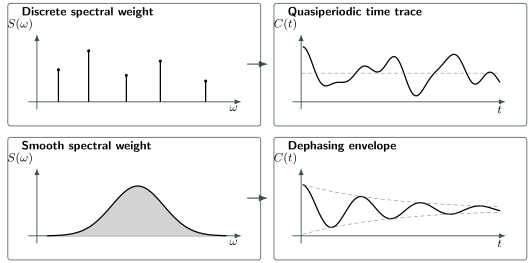

Fourier duality between spectral weight and temporal structure. A finite set of sharp frequencies produces a quasiperiodic sum with possible recurrences. A smooth band can dephase into a decaying envelope. A delta function at zero frequency would instead leave a nondecaying plateau.

The Fourier transform translates spectral structure into temporal behavior:

Spectral feature	Time-domain signature
one delta line at $\omega_0$	persistent oscillation $e^{-i\omega_0t}$
several incommensurate lines	quasiperiodic beating
exact zero-frequency delta weight	constant plateau
Lorentzian line	exponential envelope
Gaussian line	Gaussian envelope
band edge or threshold	oscillatory power-law tail
dense smooth continuum	dephasing toward zero under suitable conditions

This dictionary is not one-way proof. A finite observation window can make discrete lines look continuous, and many line shapes can approximate the same short-time curve.

Equal time as total spectral weight

Setting $t=0$ in the inverse transform gives

$$C_{AB}^{>}(0) = \int_{-\infty}^{\infty} \frac{d\omega}{2\pi}\, S_{AB}^{>}(\omega).$$

Equal-time data fix the total spectral weight but not how it is distributed in frequency.

Frequency moments

The first moment is

$$\int_{-\infty}^{\infty} \frac{d\omega}{2\pi}\, \omega S_{AB}^{>}(\omega) = \frac{1}{\hbar} \left\langle [A,H]B \right\rangle.$$

This follows either from the Lehmann sum or from differentiating at $t=0$. Higher moments involve nested commutators with $H$. These identities are exact validation checks and are developed systematically on Sum Rules.

Thermal Detailed Balance

For a canonical state,

$$\rho_\beta = \frac{e^{-\beta H}}{Z}, \qquad p_n = \frac{e^{-\beta E_n}}{Z}.$$

Define the reversed-order spectrum with the same Fourier sign:

$$S_{AB}^{<}(\omega) = \int_{-\infty}^{\infty} dt\, e^{i\omega t} \left\langle B(0)A(t) \right\rangle_\beta.$$

For $B=A^\dagger$, swapping $n$ and $m$ in the Lehmann sum gives

$$S_{AA^\dagger}^{<}(\omega) = e^{-\beta\hbar\omega} S_{AA^\dagger}^{>}(\omega).$$

At positive $\omega$, the reversed process is suppressed by the Boltzmann factor. This is detailed balance. It relates two operator orders; it does not say that one unsymmetrized spectrum is even in frequency.

The time-domain Kubo–Martin–Schwinger relation is

$$\left\langle A(t)B(0) \right\rangle_\beta = \left\langle B(0)A(t+i\beta\hbar) \right\rangle_\beta,$$

provided the analytic continuation and operator domains are well defined. This relation underlies thermal fluctuation–dissipation formulas; Fluctuation–Dissipation Theorem owns the response reconstruction, quantum factor, limiting regimes, and convention bookkeeping.

At zero temperature, a ground-state correlator with $B=A^\dagger$ has support only on transition directions allowed by the chosen order. Reversing the order reverses which side of the spectrum is populated. Calling positive frequency “absorption” without stating the operator order can therefore invert the interpretation.

Harmonic-Oscillator Benchmark

For

$$H = \hbar\omega_0 \left( a^\dagger a+\frac{1}{2} \right)$$

and

$$x = \sqrt{ \frac{\hbar}{2m\omega_0} } \left( a+a^\dagger \right),$$

the Heisenberg operator is

$$x(t) = \sqrt{ \frac{\hbar}{2m\omega_0} } \left( ae^{-i\omega_0t} + a^\dagger e^{i\omega_0t} \right).$$

In a thermal state with

$$\overline n = \frac{1}{ e^{\beta\hbar\omega_0}-1 },$$

the ordered correlator is

$$\begin{aligned} \left\langle x(t)x(0) \right\rangle_\beta ={}& \frac{\hbar}{2m\omega_0} \big[ (\overline n+1)e^{-i\omega_0t} \\ &\qquad+ \overline n e^{i\omega_0t} \big]. \end{aligned}$$

Its real and imaginary parts are

$$\begin{aligned} \operatorname{Re} \left\langle x(t)x(0) \right\rangle_\beta &= \frac{\hbar}{2m\omega_0} (2\overline n+1) \cos(\omega_0t), \\ \operatorname{Im} \left\langle x(t)x(0) \right\rangle_\beta &= - \frac{\hbar}{2m\omega_0} \sin(\omega_0t). \end{aligned}$$

The symmetric fluctuation grows with temperature, while the commutator part is state independent:

$$\left\langle [x(t),x(0)] \right\rangle = - \frac{i\hbar}{m\omega_0} \sin(\omega_0t).$$

The spectrum is

$$\begin{aligned} S_{xx}^{>}(\omega) ={}& \frac{\pi\hbar}{m\omega_0} \big[ (\overline n+1) \delta(\omega-\omega_0) \\ &\qquad+ \overline n \delta(\omega+\omega_0) \big]. \end{aligned}$$

The ratio of negative- to positive-frequency weights is

$$\frac{\overline n}{ \overline n+1 } = e^{-\beta\hbar\omega_0},$$

which is detailed balance in its simplest exact form.

Spatially Resolved Dynamics

A many-body correlator commonly retains both separation and relative time:

$$C_{AB}(\mathbf r,t) = \left\langle A_{\mathbf r}(t) B_{\mathbf 0}(0) \right\rangle.$$

It can reveal:

• propagation fronts after a local perturbation;
• ballistic, diffusive, or subdiffusive spreading;
• coherent modes and multi-particle continua;
• oscillating density, spin, or pair patterns;
• hydrodynamic long-time tails;
• relaxation toward a stationary local state.

For a density mode,

$$\rho_{\mathbf q} = \sum_j e^{-i\mathbf q\cdot\mathbf r_j} n_j,$$

an intermediate scattering function is

$$F(\mathbf q,t) = \frac{1}{N} \left\langle \rho_{\mathbf q}(t) \rho_{-\mathbf q}(0) \right\rangle.$$

Its frequency transform is a dynamic structure factor under a specified normalization. The detailed scattering interpretation, elastic pieces, and momentum conventions belong to Structure Factors.

Correlation fronts and locality

For local lattice Hamiltonians, Lieb–Robinson bounds constrain the norm of a commutator such as

$$\left\| [A_X(t),B_Y] \right\|.$$

They provide an effective causal cone for the influence of a perturbation. They do not say that an ordinary correlator must vanish outside that cone: the initial state may already contain long-range correlations. A commutator front, a connected-correlation front, and a quasiparticle group velocity are related but not identical diagnostics.

Connected Dynamical Correlations

For a stationary state,

$$C_{AB}^{>,c}(t) = \left\langle A(t)B(0) \right\rangle - \langle A\rangle \langle B\rangle.$$

The subtraction removes the static disconnected contribution, which appears as a zero-frequency delta function:

$$S_{AB}^{>}(\omega) = S_{AB}^{>,c}(\omega) + 2\pi \langle A\rangle \langle B\rangle \delta(\omega).$$

Connected subtraction does not remove every nondecaying component. Degenerate energy transitions, exact conserved projections, symmetry sectors, and integrability can leave additional zero-frequency or singular weight.

For a nonstationary state, the means themselves depend on time:

$$\begin{aligned} C_{AB}^{c}(t,t') ={}& \left\langle A(t)B(t') \right\rangle \\ &- \left\langle A(t)\right\rangle \left\langle B(t')\right\rangle. \end{aligned}$$

The later Connected Correlation Functions page owns cumulants, clustering, and asymptotic subtraction in depth.

Dephasing Is Not Irreversibility

In a finite isolated system, the Lehmann representation is a finite or countable sum of pure phases. For a finite-dimensional Hilbert space,

$$C_{AB}(t) = \sum_\ell w_\ell e^{-i\omega_\ell t}.$$

Different phases can nearly cancel over an interval, producing apparent decay. Yet unitary dynamics retains the amplitudes $w_\ell$, and the phases can partially or nearly realign. The result is generally quasiperiodic, with recurrences possible.

True smooth decay in an effective description usually invokes at least one of:

• a thermodynamic limit producing a dense spectrum;
• a continuum of scattering states;
• coarse graining or finite detector resolution;
• averaging over disorder or initial conditions;
• coupling to unobserved degrees of freedom;
• a controlled kinetic or hydrodynamic limit;
• a finite observation window that cannot resolve recurrences.

Interactions alone do not make a finite closed spectrum irreversible.

Long-time average

For a stationary finite system,

$$\overline C_{AB} = \lim_{T\to\infty} \frac{1}{T} \int_0^T dt\, C_{AB}(t)$$

selects zero transition frequency:

$$\overline C_{AB} = \sum_{n,m:\,E_n=E_m} p_n A_{nm}B_{mn}.$$

If energy levels are nondegenerate, this reduces to

$$\overline C_{AB} = \sum_n p_n A_{nn}B_{nn}.$$

This need not equal $\langle A\rangle\langle B\rangle$. A nonzero connected long-time average can reflect conserved diagonal information rather than a failure of unitary quantum mechanics.

Thermodynamic-limit order

The limits

$$\lim_{t\to\infty} \lim_{L\to\infty} C_L(t)$$

and

$$\lim_{L\to\infty} \lim_{t\to\infty} C_L(t)$$

need not agree. Taking $L\to\infty$ first can turn discrete recurrences into a continuum decay law. Taking $t\to\infty$ first at fixed $L$ retains finite-size spectral discreteness. A claim of relaxation must state the order of limits.

Line Shapes and Decay Envelopes

Consider the two-sided model

$$C(t) = C_0 e^{-i\omega_0t} e^{-\Gamma\lvert t\rvert}.$$

With the Fourier convention on this page,

$$S(\omega) = \frac{ 2C_0\Gamma }{ (\omega-\omega_0)^2+\Gamma^2 }.$$

The half width at half maximum is $\Gamma$, and the envelope time is $1/\Gamma$. This reciprocal relation relies on the exponential and Lorentzian model. A Gaussian envelope, stretched exponential, power law, finite-support spectrum, or multi-line spectrum has a different width–time dictionary.

Threshold nonanalyticities often produce oscillatory power-law tails. If spectral weight begins near $\omega_{\mathrm{th}}$ as

$$S(\omega) \sim (\omega-\omega_{\mathrm{th}})^\alpha \theta(\omega-\omega_{\mathrm{th}}),$$

then under suitable regularity assumptions its long-time transform contains

$$C(t) \sim e^{-i\omega_{\mathrm{th}}t} t^{-(\alpha+1)}$$

up to a phase and coefficient. Long-time dynamics is therefore especially sensitive to sharp spectral edges and conserved low-frequency structure.

What a Correlation Time Means

There is no universal correlation time. Common definitions include:

Exponential fit

If

$$C^c(t) \approx C^c(0)e^{-t/\tau}$$

over a justified range, $\tau$ is the fitted envelope time. Oscillations, multiple rates, and finite offsets must be modeled rather than silently discarded.

Integrated correlation time

For a real normalized stationary correlator,

$$\tau_{\mathrm{int}} = \int_0^\infty dt\, \frac{C^c(t)}{C^c(0)}.$$

Oscillatory cancellation can make this small or even negative. Some applications instead integrate the absolute value or square, producing a different quantity.

Spectral linewidth

A linewidth can define a time only after choosing:

• angular frequency versus ordinary frequency;
• full width versus half width;
• amplitude decay versus intensity decay;
• intrinsic width versus instrumental or window broadening;
• a specific line shape.

A nondecaying plateau makes an unmodified integral diverge. A power-law tail may also make the correlation time infinite even though $C(t)\to0$.

Conserved Components

If $A$ commutes with $H$,

$$[H,A] = 0,$$

then

$$A(t) = A$$

and

$$C_{AB}^{>}(t) = \left\langle AB \right\rangle$$

is constant. Its spectrum is entirely at zero frequency:

$$S_{AB}^{>}(\omega) = 2\pi \left\langle AB \right\rangle \delta(\omega).$$

More generally, decompose

$$A = A_\parallel + A_\perp,$$

where $A_\parallel$ is the projection onto operators conserved under the dynamics. The $A_\parallel$ component produces persistent weight, while $A_\perp$ may dephase.

A vanishing retarded self-response of an exactly conserved quantity is compatible with a nonzero ordinary autocorrelation: the commutator can vanish while the fluctuation remains. Response and fluctuation are not interchangeable outside a carefully stated equilibrium relation.

Nonequilibrium Two-Time Structure

For a nonstationary state, introduce center and relative times:

$$T = \frac{t+t'}{2}, \qquad \tau = t-t'.$$

Then

$$C_{AB}(t,t') = C_{AB} \left( T+\frac{\tau}{2}, T-\frac{\tau}{2} \right).$$

A Wigner transform Fourier transforms only the relative time:

$$\begin{aligned} C_{AB}(T,\omega) ={}& \int_{-\infty}^{\infty} d\tau\, e^{i\omega\tau} \\ &\times C_{AB} \left( T+\frac{\tau}{2}, T-\frac{\tau}{2} \right). \end{aligned}$$

The center time tracks slow evolution of the background; $\omega$ resolves relative-time oscillations. Interpreting $C(T,\omega)$ as an instantaneous spectrum requires scale separation. Without it, time and frequency resolution compete, and a cross-Wigner distribution can be complex or sign-indefinite.

Quenches

After a sudden change of Hamiltonian, $\rho_0$ generally has off-diagonal matrix elements in the post-quench energy basis. Those coherences make a simultaneous time shift observable. At late times, local observables may approach stationary values through dephasing, but the full pure state remains unitary and finite systems recur. Quantum Quenches develops the underlying switch, final-energy weights, equal-time fronts, entanglement growth, and return amplitude.

The diagonal ensemble, generalized Gibbs descriptions, and eigenstate thermalization address when selected observables become stationary. They do not imply that every two-time correlator immediately acquires an equilibrium KMS relation.

Nonequilibrium Overview develops the complementary one-time and reduced-state criteria for equilibration, thermalization, retained memory, and order of limits.

Periodic driving

In a periodic steady regime with drive period $T_d$,

$$C(t+T_d,t'+T_d) = C(t,t')$$

can hold without continuous time-translation invariance. The correlator depends on relative time and on the center-time phase within the drive cycle. A Floquet-frequency representation then contains sidebands and harmonic indices rather than one equilibrium spectrum.

Open systems

For nonunitary reduced dynamics, Heisenberg evolution is generated by the adjoint quantum channel or Liouvillian rather than by $e^{iHt/\hbar}Ae^{-iHt/\hbar}$. Multi-time correlations are not determined by the one-time reduced state alone.

The quantum regression theorem supplies a useful propagation rule under specific Markovian assumptions. Applying it to a non-Markovian bath without justification can give incorrect temporal correlations even when the one-time master equation looks accurate.

Measurement Interpretation

Time-dependent correlations require an operational protocol.

Scattering and spectroscopy

Inelastic neutron, x-ray, light, and matter-wave scattering resolve momentum and energy transfer. Cross sections contain dynamic density or spin correlations together with form factors, polarization factors, detailed-balance conventions, and instrumental resolution.

Sequential measurements

A sequence of strong projective measurements generally disturbs the state. The observed joint probability is not automatically the unmeasured operator product $\langle A(t)B(t')\rangle$.

Accessing an ordinary correlator can require weak coupling, ancilla interferometry, repeated preparation with controlled insertions, or a scattering protocol whose perturbative expansion identifies the desired order.

Destructive snapshots

If detection destroys the sample, unequal-time density correlations cannot be formed by observing one realization twice. Repeated runs with identical preparation estimate separate-time ensembles, and protocol drift becomes part of the uncertainty budget.

Detector response

A measured signal is often

$$C_{\mathrm{meas}}(t) = \int dt'\, R(t-t') C_{\mathrm{true}}(t'),$$

where $R$ is an impulse-response or timing-resolution kernel. In frequency space this convolution becomes multiplication. Detector bandwidth can imitate physical temporal decay or suppress high-frequency weight.

Numerical Evaluation

The methods below are oriented here by the correlation function they approximate. Dynamical Correlation Functions Numerically owns their detailed comparison, matched-kernel identities, convergence ladder, and reproducibility record.

Exact diagonalization

The Lehmann sum is exact once eigenvalues and matrix elements are known. It is efficient for small systems and exposes selection rules, but the spectrum consists of delta lines. A chosen Lorentzian width is a plotting or modeling parameter, not an intrinsic lifetime.

For larger sparse systems, one may compute

$$C_{AB}(t) = \langle\Psi\rvert e^{iHt/\hbar} A e^{-iHt/\hbar} B \lvert\Psi\rangle$$

using Krylov time evolution without full diagonalization. Operator order must be implemented from right to left.

Tensor networks

Real-time matrix-product-state methods can evaluate local correlators in one dimension. Entanglement growth often limits the reachable time, which in turn limits spectral resolution. Linear prediction or extrapolation can extend a signal but adds model assumptions that must be tested on controlled data.

Quantum Monte Carlo

Equilibrium Monte Carlo naturally accesses imaginary-time correlators. Recovering a real-frequency spectrum requires analytic continuation, an ill-conditioned inverse problem. Maximum entropy, stochastic continuation, and related methods impose priors or regularization; agreement with noisy imaginary-time data does not uniquely determine sharp real-frequency features.

Nonequilibrium solvers

Keldysh, tensor-network, dynamical mean-field, semiclassical, and kinetic methods compute different approximations to two-time functions. A reliable comparison states:

• the contour or operator ordering;
• whether the result is full or connected;
• the initial state and switch-on protocol;
• finite-size and time-step errors;
• conservation-law and equal-time checks;
• any self-energy, memory, or closure approximation.

Finite-Time Fourier Analysis

Numerical and experimental data cover a finite interval. A windowed transform is

$$S_T(\omega) = \int_{-T/2}^{T/2} dt\, w(t) e^{i\omega t} C(t).$$

Multiplication by $w(t)$ in time convolves the true spectrum with the transform of the window. Consequences include:

• frequency resolution of order $2\pi/T$;
• leakage from sharp lines into nearby bins;
• a tradeoff between narrow main lobes and suppressed side lobes;
• distortion of low-frequency weight by baseline subtraction;
• artificial broadening that should not be called a lifetime.

With time step $\Delta t$, the Nyquist angular frequency is

$$\omega_{\mathrm{Ny}} = \frac{\pi}{\Delta t}.$$

Frequencies above it alias into the sampled band. Zero padding gives a smoother interpolation of the discrete transform but does not improve the physical resolution set by $T$.

For a stationary Hermitian autocorrelator, enforcing the exact relation

$$C(-t) = C(t)^*$$

can reduce noise only after independently checking that stationarity and Hermiticity apply. It should not be used to conceal a broken convention.

Validation Checklist

A trustworthy result should satisfy the applicable checks:

1. $C_{AB}(t,t')$ reduces to the known equal-time value at $t=t'$.
2. A stationary calculation depends only on $t-t'$.
3. Hermitian-conjugation identities hold before optional symmetrization.
4. $S_{AA^\dagger}^{>}(\omega)$ is nonnegative within numerical uncertainty.
5. The integrated spectrum reproduces $C(0)$.
6. Low spectral moments reproduce commutator identities.
7. Thermal spectra satisfy detailed balance.
8. Exact conserved components appear at zero frequency.
9. Selection-rule zeros agree with symmetry.
10. Finite-system data show discrete lines before artificial broadening.
11. Results converge with time step, maximum time, window, size, and truncation.
12. Claimed decay survives separation from detector and analysis kernels.

Common Mistakes

• Setting one time to zero without establishing stationarity.
• Calling $\langle A(t)B(0)\rangle$ real because $A$ and $B$ are Hermitian.
• Swapping greater and lesser operator orders.
• Importing a retarded Green-function factor of $-i$ into an ordinary correlation.
• Treating an ordinary correlator as a response without a commutator and source convention.
• Calling the unsymmetrized thermal spectrum even in frequency.
• Reversing the detailed-balance exponent by changing Fourier signs halfway through.
• Reading absolute energies rather than energy differences from a Lehmann spectrum.
• Ignoring matrix-element selection rules.
• Interpreting finite-size dephasing as irreversible decay.
• Treating chosen Lorentzian broadening as a physical lifetime.
• Ignoring a zero-frequency plateau before defining a correlation time.
• Assuming interactions alone eliminate recurrences.
• Taking long-time and thermodynamic limits without stating their order.
• Applying a one-frequency equilibrium spectrum to a quench or driven state.
• Applying the quantum regression theorem outside its Markovian domain.
• Interpreting a Wigner transform as a positive instantaneous probability.
• Claiming improved resolution from zero padding.
• Ignoring aliasing, leakage, and the detector response kernel.
• Applying Wick factorization to a non-Gaussian initial state without checking it.

Reliable Workflow

1. Specify $H$, $\rho$, $A$, $B$, and the literal operator order.
2. Decide whether the state and dynamics are stationary.
3. State the Fourier sign, normalization, and use of $\omega$ versus energy.
4. Derive symmetry and conservation constraints before computing.
5. Check equal-time normalization and Hermitian conjugation.
6. Use the Lehmann representation to interpret frequencies, populations, and matrix elements.
7. Separate disconnected, conserved, and genuinely decaying pieces.
8. Distinguish finite-size dephasing from continuum relaxation.
9. Map the desired operator product to the actual measurement or numerical estimator.
10. Vary time window, step, broadening, system size, and truncation independently.
11. Test detailed balance or nonequilibrium two-time structure as appropriate.
12. Assign a correlation time only after declaring its operational definition.

Exercises

Exercise 1: Stationary reduction

Prove that

$$C_{AB}(t,t') = C_{AB}(t-t',0)$$

when $[H,\rho]=0$.

Solution

Write

$$\begin{aligned} A_H(t)B_H(t') ={}& e^{iHt'/\hbar} A_H(t-t') B e^{-iHt'/\hbar}. \end{aligned}$$

Therefore

$$\begin{aligned} C_{AB}(t,t') ={}& \operatorname{Tr} \left[ \rho e^{iHt'/\hbar} A_H(t-t')B e^{-iHt'/\hbar} \right]. \end{aligned}$$

Cyclicity moves the final unitary to the front:

$$\begin{aligned} C_{AB}(t,t') ={}& \operatorname{Tr} \left[ e^{-iHt'/\hbar} \rho e^{iHt'/\hbar} A_H(t-t')B \right]. \end{aligned}$$

Since $[H,\rho]=0$,

$$e^{-iHt'/\hbar} \rho e^{iHt'/\hbar} = \rho.$$

The result is $\operatorname{Tr}[\rho A_H(t-t')B]$, which equals $C_{AB}(t-t',0)$.

Exercise 2: Hermitian autocorrelation symmetry

Let $A=A^\dagger$ and $\rho$ be stationary. Show that

$$C_{AA}(t)^* = C_{AA}(-t).$$

Deduce the parity of its real and imaginary parts.

Solution

Complex conjugation gives

$$\begin{aligned} C_{AA}(t)^* &= \left\langle A(t)A(0) \right\rangle^* \\ &= \left\langle A(0)A(t) \right\rangle. \end{aligned}$$

Stationarity permits a common shift by $-t$:

$$\left\langle A(0)A(t) \right\rangle = \left\langle A(-t)A(0) \right\rangle = C_{AA}(-t).$$

Writing $C(t)=R(t)+iI(t)$ and comparing both sides gives

$$R(t) = R(-t), \qquad I(t) = -I(-t).$$

Thus the real part is even and the imaginary part is odd.

Exercise 3: Harmonic-oscillator detailed balance

Starting from

$$x(t) = \sqrt{ \frac{\hbar}{2m\omega_0} } \left( ae^{-i\omega_0t} + a^\dagger e^{i\omega_0t} \right),$$

derive the thermal $S_{xx}^{>}(\omega)$ and verify the ratio of its negative- and positive-frequency weights.

Solution

The thermal contractions are

$$\left\langle a^\dagger a \right\rangle = \overline n, \qquad \left\langle aa^\dagger \right\rangle = \overline n+1,$$

while $\langle aa\rangle=\langle a^\dagger a^\dagger\rangle=0$. Hence

$$\begin{aligned} C_{xx}^{>}(t) ={}& \frac{\hbar}{2m\omega_0} \big[ (\overline n+1)e^{-i\omega_0t} \\ &\qquad+ \overline n e^{i\omega_0t} \big]. \end{aligned}$$

Using

$$\int_{-\infty}^{\infty} dt\, e^{i(\omega-\omega_0)t} = 2\pi\delta(\omega-\omega_0),$$

we obtain

$$\begin{aligned} S_{xx}^{>}(\omega) ={}& \frac{\pi\hbar}{m\omega_0} \big[ (\overline n+1)\delta(\omega-\omega_0) \\ &\qquad+ \overline n\delta(\omega+\omega_0) \big]. \end{aligned}$$

Since

$$\overline n = \frac{1}{ e^{\beta\hbar\omega_0}-1 },$$

the ratio is

$$\frac{\overline n}{ \overline n+1 } = e^{-\beta\hbar\omega_0}.$$

Exercise 4: Long-time average

For

$$C_{AB}(t) = \sum_{n,m} p_n e^{i(E_n-E_m)t/\hbar} A_{nm}B_{mn},$$

compute the infinite-time average. What changes when the spectrum is degenerate?

Solution

Each phase contributes

$$\frac{1}{T} \int_0^T dt\, e^{i(E_n-E_m)t/\hbar}.$$

As $T\to\infty$, this tends to zero when $E_n\ne E_m$ and to one when $E_n=E_m$. Therefore

$$\overline C_{AB} = \sum_{n,m:\,E_n=E_m} p_n A_{nm}B_{mn}.$$

For a nondegenerate spectrum, only $m=n$ remains:

$$\overline C_{AB} = \sum_n p_n A_{nn}B_{nn}.$$

With degeneracy, off-diagonal matrix elements inside a common-energy block can survive. One may diagonalize $\rho$ inside the block, but $A$ and $B$ need not be diagonal there.

Exercise 5: Exponential envelope and Lorentzian line

Evaluate the Fourier transform of

$$C(t) = C_0 e^{-i\omega_0t} e^{-\Gamma\lvert t\rvert}, \qquad \Gamma>0.$$

Solution

Split the integral at $t=0$:

$$\begin{aligned} S(\omega) ={}& C_0 \int_0^\infty dt\, e^{-[\Gamma-i(\omega-\omega_0)]t} \\ &+ C_0 \int_0^\infty dt\, e^{-[\Gamma+i(\omega-\omega_0)]t}. \end{aligned}$$

The two terms are

$$\frac{C_0}{ \Gamma-i(\omega-\omega_0) }$$

and its complex conjugate. Their sum is

$$S(\omega) = \frac{ 2C_0\Gamma }{ (\omega-\omega_0)^2+\Gamma^2 }.$$

At $\omega=\omega_0\pm\Gamma$, the value is half the peak value. Thus $\Gamma$ is the half width at half maximum for this convention.

Exercise 6: Conserved autocorrelation and zero-frequency weight

Suppose $[H,A]=0$. Show that $C_{AA^\dagger}^{>}(t)$ is constant and find its spectrum. What is the retarded self-response?

Solution

Conservation gives

$$A(t) = A.$$

Therefore

$$C_{AA^\dagger}^{>}(t) = \left\langle AA^\dagger \right\rangle.$$

The Fourier transform of a constant is

$$S_{AA^\dagger}^{>}(\omega) = 2\pi \left\langle AA^\dagger \right\rangle \delta(\omega).$$

The retarded self-response built from $[A(t),A]$ vanishes if $A$ is Hermitian, because the commutator is zero. A persistent ordinary fluctuation and a vanishing isolated response are therefore compatible.

Exercise 7: Stationary Wigner transform

Suppose

$$C(t,t') = C(t-t').$$

Show that its Wigner transform is independent of center time $T$ and reduces to the ordinary spectrum.

Solution

By definition,

$$\begin{aligned} C(T,\omega) ={}& \int_{-\infty}^{\infty} d\tau\, e^{i\omega\tau} \\ &\times C \left( T+\frac{\tau}{2}, T-\frac{\tau}{2} \right). \end{aligned}$$

Stationarity makes the two-time argument depend only on

$$\left( T+\frac{\tau}{2} \right) - \left( T-\frac{\tau}{2} \right) = \tau.$$

Hence

$$C(T,\omega) = \int_{-\infty}^{\infty} d\tau\, e^{i\omega\tau} C(\tau) = S(\omega),$$

with no $T$ dependence.

Exercise 8: Sampling limits

A real-time signal is sampled every $\Delta t$ over a total duration $T$. State the Nyquist angular frequency and the scale of the Fourier resolution. Does zero padding improve either?

Solution

Sampling at interval $\Delta t$ identifies frequencies that differ by integer multiples of

$$\frac{2\pi}{\Delta t}.$$

The nonaliased angular-frequency band can be chosen as

$$-\frac{\pi}{\Delta t} \leq \omega < \frac{\pi}{\Delta t},$$

so

$$\omega_{\mathrm{Ny}} = \frac{\pi}{\Delta t}.$$

A total duration $T$ gives a characteristic bin spacing and physical resolution of order

$$\Delta\omega \sim \frac{2\pi}{T},$$

with the exact line shape set by the window. Zero padding evaluates the same finite-window transform on a denser frequency grid. It improves visual interpolation but changes neither Nyquist bandwidth nor physical resolution.

Cross-Links

• Correlation Functions Overview — hierarchy, decay regimes, and ordering map.
• Equal-Time Correlations — static limit and equal-time operator diagnostics.
• Structure Factors — momentum–frequency spectra and scattering probes.
• Green Functions in Many-Body QM — number-changing propagators and addition/removal spectra.
• Retarded and Advanced Response — causal commutator response and its advanced boundary partner.
• Spectral Functions — exact lines, continua, linewidths, and finite-resolution interpretation.
• Dynamical Correlation Functions Numerically — direct, Krylov, and time-domain numerical routes with controlled resolution.
• Fluctuation–Dissipation Theorem — KMS balance and the conversion between fluctuations and absorption.
• Sum Rules — short-time derivatives, spectral moments, and nested commutators.
• Correlation Functions Formula Card — compact convention lookup.
• Heisenberg Picture — operator evolution and equations of motion.
• Stationary States and Phases — stationary-state phase evolution and recurrence.
• Thermal Density Operators — equilibrium states and energy-basis weights.
• Kubo Formula — retarded response, causal signs, and source conventions.
• Spectral Representation of Green Functions — propagator and resolvent spectra.
• Retarded and Advanced Green Functions — boundary conditions and the $i0$ prescription.
• Correlation Functions in Path Integrals — time-ordered source insertions.
• Bath Correlation Functions — environmental memory and master-equation rates.
• Noise Spectra — ordered and symmetrized environmental spectra.
• Thermodynamic Limit — recurrence and the order of large-system and long-time limits.

References

1. A. L. Fetter and J. D. Walecka, Quantum Theory of Many-Particle Systems, Dover (2003).
2. J. W. Negele and H. Orland, Quantum Many-Particle Systems, Westview Press (1998).
3. G. D. Mahan, Many-Particle Physics, 3rd ed., Springer (2000).
4. P. Coleman, Introduction to Many-Body Physics, Cambridge University Press (2015).
5. A. Altland and B. Simons, Condensed Matter Field Theory, 2nd ed., Cambridge University Press (2010).
6. L. Van Hove, “Correlations in Space and Time and Born Approximation Scattering in Systems of Interacting Particles”, Physical Review 95, 249–262 (1954).
7. H. Lehmann, “On the Properties of Propagation Functions and Renormalization Constants of Quantized Fields”, Il Nuovo Cimento 11, 342–357 (1954).
8. R. Kubo, “Statistical-Mechanical Theory of Irreversible Processes. I. General Theory and Simple Applications to Magnetic and Conduction Problems”, Journal of the Physical Society of Japan 12, 570–586 (1957).
9. P. C. Martin and J. Schwinger, “Theory of Many-Particle Systems. I”, Physical Review 115, 1342–1373 (1959).
10. E. H. Lieb and D. W. Robinson, “The Finite Group Velocity of Quantum Spin Systems”, Communications in Mathematical Physics 28, 251–257 (1972).
11. S. R. White and A. E. Feiguin, “Real-Time Evolution Using the Density Matrix Renormalization Group”, Physical Review Letters 93, 076401 (2004).
12. A. J. Daley, C. Kollath, U. Schollwöck, and G. Vidal, “Time-Dependent Density-Matrix Renormalization-Group Using Adaptive Effective Hilbert Spaces”, Journal of Physics A 37, 10391–10407 (2004).
13. M. Rigol, V. Dunjko, and M. Olshanii, “Thermalization and Its Mechanism for Generic Isolated Quantum Systems”, Nature 452, 854–858 (2008).