Dynamical Correlation Functions Numerically

A numerical spectrum is trustworthy only when the exact target, the algorithmic approximation, and the displayed line shape are kept distinct. Direct Lehmann sums, Lanczos continued fractions, and real-time Fourier transforms can represent the same finite-system correlation function, but they distribute cost and error very differently.

For a finite isolated system, the exact answer is usually a weighted set of delta functions. Smooth curves arise only after a declared resolution operation, a physical broadening mechanism, or a controlled thermodynamic limit. The central evidence chain is therefore

$$\begin{gathered} \text{declared target} \longrightarrow \text{finite measure} \\ \text{algorithm} \longrightarrow \text{resolved estimator} \\ \text{size scaling} \longrightarrow \text{qualified claim}. \end{gathered}$$

This page develops that chain as a computational workflow.

Purpose and Canonical Scope

This page is the canonical home for the numerical comparison and validation of stationary dynamical correlations in finite many-body systems. It owns:

• the common input and output contract for direct Lehmann, Lanczos, and real-time calculations;
• method selection by spectral window, system size, representation, and desired resolution;
• the separation of ground-state, propagation, Krylov, truncation, sampling, and broadening errors;
• cross-method identities that turn one algorithm into a benchmark for another;
• frequency-resolution and finite-size scaling protocols;
• reproducibility records for numerical spectra.

Neighboring pages retain their more fundamental or method-specific topics:

• Time-Dependent Correlations owns operator ordering, stationarity, Lehmann physics, dephasing, recurrence, and finite-time Fourier theory.
• Spectral Functions owns the dictionary among spectral objects, poles, continua, line shapes, residues, linewidths, and experimental forward models.
• Lanczos Method Preview owns the Krylov recurrence, Ritz-state certification, continued-fraction derivation, and finite-precision Lanczos failures.
• Exact Diagonalization Preview owns basis construction, complete versus targeted diagonalization, and finite-space interpretation.
• Sum Rules owns the exact moment hierarchy and nested-commutator derivations.
• Analytic Continuation owns reconstruction of real-frequency information from imaginary-time data.
• Tensor Networks: Computational Guide and DMRG Preview own finite-bond convergence and ground-state optimization.

The main setting below is a zero-temperature stationary correlator of a finite Hermitian Hamiltonian. Thermal traces, nonequilibrium two-time functions, and open-system spectra require additional state and contour choices, but the same error-accounting principles remain useful.

Declare the Target Before the Method

Let

$$H|n\rangle = E_n|n\rangle, \qquad E_n\ge E_0,$$

and suppose a normalized ground state $|0\rangle$ has been selected within a declared symmetry sector. For an operator $A$, define the connected insertion

$$\widetilde A = A-\langle0|A|0\rangle.$$

The response seed is

$$|f_0\rangle = \widetilde A|0\rangle, \qquad W_0 = \langle f_0|f_0\rangle.$$

Subtracting the expectation value removes the elastic ground-state contribution for this autocorrelation channel. It does not remove other exactly zero-energy transitions caused by degeneracy or conserved components.

This page uses energy transfer $E$, not angular frequency, as the spectral variable:

$$E = \hbar\omega.$$

The positive spectral measure and its time-domain partner are

$$\begin{aligned} S_A(E) &= \sum_n |\langle n|\widetilde A|0\rangle|^2 \delta\!\left( E-E_n+E_0 \right), \\ C_A(t) &= \langle f_0| e^{-i(H-E_0)t/\hbar} |f_0\rangle. \end{aligned}$$

With these conventions,

$$\begin{aligned} C_A(t) &= \int_0^\infty dE\, S_A(E)e^{-iEt/\hbar}, \\ S_A(E) &= \frac{1}{2\pi\hbar} \int_{-\infty}^{\infty} dt\, e^{iEt/\hbar}C_A(t). \end{aligned}$$

The declaration of a numerical task should record at least

$$\begin{aligned} \mathcal D = \bigl( &H,\, \mathcal H_{\lambda_0},\, |0\rangle,\, \widetilde A, \\ &\mathcal H_{\lambda_A},\, \mathcal I_E,\, \delta E_{\mathrm{target}} \bigr), \end{aligned}$$

where $\mathcal H_{\lambda_0}$ is the ground-state sector, $\mathcal H_{\lambda_A}$ is the sector reached by $\widetilde A$, $\mathcal I_E$ is the energy window of interest, and $\delta E_{\mathrm{target}}$ is the requested resolution.

Without this declaration, the phrase “compute the spectrum” leaves the physical channel, accessible states, and numerical target unspecified.

Three Different Outputs

One calculation can produce three mathematically different objects.

Exact finite-system measure

For finite dimension,

$$S_{A,L}(E) = \sum_j w_{j,L} \delta(E-\varepsilon_{j,L}),$$

where $L$ labels the finite geometry. The pole positions and weights are exact only for the represented finite Hamiltonian and state.

Algorithmic approximation

An iterative method returns approximations such as

$$\begin{gathered} \left\{ \widetilde\varepsilon_j,\, \widetilde w_j \right\}, \qquad \widetilde C(t_k), \\ \text{or} \qquad \widetilde G(E+i\eta). \end{gathered}$$

These carry solver, propagation, truncation, and floating-point errors before any physical limit is considered.

Displayed or regularized spectrum

A plotted function is commonly

$$\widetilde S_{A,L,K}(E) = \int dE'\, K(E-E') \widetilde S_{A,L}(E'),$$

for a declared kernel $K$. Its peak widths include the chosen kernel even when the exact finite-system lines have zero intrinsic width.

These objects answer different questions. Convergence of the algorithmic approximation does not establish convergence in $L$, and visual smoothness does not establish an intrinsic continuum.

Method Map

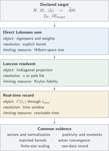
Direct Lehmann sums, Lanczos projection, and real-time propagation approximate the same operator-resolved measure through different intermediate objects. Their outputs become comparable only after the finite problem, resolution kernel, and validation tests are matched.

Route	Primary computed object	Natural strength	Dominant limitation
direct Lehmann sum	eigenvalues and matrix elements	exact finite benchmark and all operators after diagonalization	exponential state count and eigenvector storage
Lanczos response	projected resolvent or tridiagonal poles	many frequencies from one operator seed	Krylov convergence, loss of orthogonality, finite-size poles
real-time evolution	sampled overlap $C_A(t_k)$	broad spectral window and space-time data	reachable time, time step, recurrence, entanglement growth
correction vector	response state at selected $E+i\eta$	controlled narrow frequency windows	one difficult linear solve per frequency or block
polynomial expansion	spectral moments	uniform broad windows with explicit kernels	rescaling, recursion order, moment stability

The first three routes are developed in detail below. The final two are included to prevent a false three-method taxonomy: they can be preferable when the desired frequency window or representation makes them a better match.

Direct Lehmann Sums

Complete diagonalization gives the finite-system spectrum most literally:

$$\varepsilon_n = E_n-E_0, \qquad w_n = |\langle n|\widetilde A|0\rangle|^2.$$

The workflow is:

1. construct and verify the finite Hamiltonian;
2. diagonalize the ground-state sector;
3. apply $\widetilde A$ to determine the destination sector;
4. diagonalize every destination-sector state needed in the requested window;
5. evaluate matrix elements and preserve the unbroadened line list;
6. verify exact identities before choosing a display kernel.

The zeroth and first moments are

$$\begin{aligned} \mu_0 &= \sum_n w_n = \langle0| \widetilde A^\dagger\widetilde A |0\rangle, \\ \mu_1 &= \sum_n w_n\varepsilon_n \\ &= \langle0| \widetilde A^\dagger (H-E_0) \widetilde A |0\rangle. \end{aligned}$$

For Hermitian $\widetilde A$, the first moment can also be related to a double commutator under the conventions developed on Sum Rules.

Sector bookkeeping

If $A$ carries conserved quantum numbers $\Delta\lambda_A$, then

$$\widetilde A: \mathcal H_{\lambda_0} \longrightarrow \mathcal H_{\lambda_0+\Delta\lambda_A}.$$

A spin-raising operator changes total magnetization, a creation operator changes particle number, and a momentum-resolved operator changes crystal momentum. The destination basis may therefore differ from the ground-state basis.

A vanishing matrix element can be a physical selection rule, but it can also signal that the operator was represented in the wrong sector. The numerical record should distinguish those possibilities.

Degenerate destination states

Individual weights inside an exactly degenerate eigenspace depend on the basis chosen within that space. The total weight does not. For the projector $P_{\mathcal D}$ onto a degenerate block,

$$W_{\mathcal D} = \langle0| \widetilde A^\dagger P_{\mathcal D} \widetilde A |0\rangle$$

is basis invariant. Compare block weights rather than individual eigenvector labels when eigensolvers rotate a degenerate subspace.

When direct Lehmann is the right tool

Use direct sums when:

• the full relevant sector is small enough to diagonalize and retain;
• many different operators will be evaluated on the same eigenbasis;
• exact thermal traces are required in a small system;
• a benchmark is needed for iterative or compressed-state methods;
• individual finite-size poles and selection rules are themselves the target.

Do not call a partial eigensystem a complete Lehmann sum. Missing high-energy states can violate normalization and moment identities even when the low-energy plot looks plausible.

A Common Three-Level Benchmark

Consider an operator-generated state supported on two exact excitations:

$$|f_0\rangle = \frac{\sqrt3}{2}|1\rangle + \frac12|2\rangle,$$

with

$$\begin{aligned} (H-E_0)|1\rangle &= \Delta|1\rangle, \\ (H-E_0)|2\rangle &= 3\Delta|2\rangle. \end{aligned}$$

The exact line measure is

$$S(E) = \frac34\delta(E-\Delta) + \frac14\delta(E-3\Delta),$$

and the exact correlator is

$$C(t) = \frac34e^{-i\Delta t/\hbar} + \frac14e^{-i3\Delta t/\hbar}.$$

The first moments are

$$\mu_0=1, \qquad \mu_1=\frac32\Delta, \qquad \mu_2=3\Delta^2.$$

This tiny problem is useful because every numerical route must reproduce the same weights, phases, and moments while exposing its own approximation.

Lanczos Continued Fractions

A response Lanczos run starts from

$$|q_1\rangle = \frac{|f_0\rangle}{\sqrt{W_0}}$$

and projects $H-E_0$ onto the Krylov space generated by repeated Hamiltonian action. If $T_m$ is the resulting $m\times m$ tridiagonal matrix, then

$$\begin{gathered} G_A^{(m)}(z) = W_0 e_1^{\mathsf T} (zI_m-T_m)^{-1} e_1, \\ \operatorname{Im}z>0. \end{gathered}$$

Expanding this matrix element gives the familiar continued fraction. Its derivation, indexing, residual logic, and finite-precision safeguards belong to Lanczos Method Preview.

Diagonalizing the small $T_m$ gives

$$G_A^{(m)}(z) = \sum_{\ell=1}^{m} \frac{w_\ell^{(m)}} {z-\vartheta_\ell^{(m)}},$$

where

$$w_\ell^{(m)} = W_0 |(y_\ell)_1|^2 \ge0.$$

One response run therefore supplies a compact pole representation that can be evaluated on many frequency grids and for many choices of $\eta$ without repeating Hamiltonian-vector products.

What converges first

Lanczos is a moment method as well as a pole method. In exact arithmetic,

$$\mu_p = W_0 e_1^{\mathsf T} T_m^p e_1$$

is exact through a method-dependent range that reaches $p=2m-1$ before early termination. Integrated spectral information can therefore converge before every visible pole.

This creates two opposite mistakes:

• rejecting a useful response because individual high-energy poles still move even though the target moments and broadened window are stable;
• accepting a detailed line assignment merely because low moments are correct.

Convergence must be tested at the level of the claimed observable.

Benchmark termination

For the three-level benchmark, the first diagonal coefficient and off-diagonal coefficient are

$$\alpha_1 = \frac32\Delta, \qquad \beta_2 = \frac{\sqrt3}{2}\Delta.$$

The second diagonal coefficient is

$$\alpha_2 = \frac52\Delta.$$

Thus

$$T_2 = \Delta \begin{pmatrix} 3/2 & \sqrt3/2 \\ \sqrt3/2 & 5/2 \end{pmatrix},$$

whose eigenvalues are $\Delta$ and $3\Delta$ with the exact spectral weights $3/4$ and $1/4$. The Krylov space has exhausted the support of $|f_0\rangle$, so the response terminates exactly after two basis vectors even if the full Hilbert space is larger.

Error ledger for a Lanczos spectrum

Keep at least four errors separate:

1. Reference-state error: $E_0$ and $|0\rangle$ may be approximate.
2. Response-Krylov error: finite $m$ limits the represented moments and pole detail.
3. Finite-precision error: loss of orthogonality can create duplicate or unstable poles.
4. Resolution choice: evaluating $z=E+i\eta$ convolves the discrete measure with a Lorentzian.

Increasing $m$ does not remove ground-state bias, finite-size effects, or the chosen $\eta$. Decreasing $\eta$ can reveal unconverged Krylov poles rather than more physics.

Real-Time Evolution and Fourier Transform

The time-domain route propagates the same response seed:

$$|f(t)\rangle = e^{-i(H-E_0)t/\hbar} |f_0\rangle,$$

then evaluates

$$C_A(t) = \langle f_0|f(t)\rangle.$$

The propagation may use exact exponentiation in a tiny space, a Krylov exponential, product formulas, matrix-product-state evolution, or another controlled representation. Those algorithms have different internal errors, but the spectral reconstruction sees only the accuracy and duration of the resulting time record.

Sampled record

Let

$$\begin{gathered} t_j = j\Delta t, \qquad j=0,\ldots,N, \\ t_{\max} = N\Delta t. \end{gathered}$$

For a stationary Hermitian autocorrelation,

$$C_A(-t) = C_A(t)^*,$$

so a verified positive-time record can be extended to a total interval of length approximately $2t_{\max}$. The associated scales are

$$\begin{aligned} E_{\mathrm{Ny}} &= \frac{\pi\hbar}{\Delta t}, \\ \delta E_{\mathrm{grid}} &\simeq \frac{\pi\hbar}{t_{\max}}. \end{aligned}$$

The second quantity is a frequency-grid scale for the symmetrically extended record, not a universal resolving power. The main-lobe width of the chosen window is the relevant resolution measure.

Windowed transform

For an even time window $w(t)$ supported on $[-t_{\max},t_{\max}]$, define

$$\widetilde S_w(E) = \frac{1}{2\pi\hbar} \int_{-t_{\max}}^{t_{\max}} dt\, w(t)e^{iEt/\hbar} \widetilde C_A(t).$$

If propagation were exact and the interval infinite, multiplication in time would give convolution in energy:

$$\widetilde S_w(E) = \int dE'\, K_w(E-E') S_A(E'),$$

with

$$K_w(E) = \frac{1}{2\pi\hbar} \int dt\, w(t)e^{iEt/\hbar}.$$

The window is therefore part of the spectral estimator, not cosmetic post-processing.

Two useful infinite-time kernels

Exponential damping,

$$w_\eta(t) = e^{-\eta|t|/\hbar},$$

produces the normalized Lorentzian

$$K_\eta(E) = \frac1\pi \frac{\eta}{E^2+\eta^2}.$$

Gaussian damping,

$$w_\sigma(t) = \exp\!\left[ -\frac12 \left( \frac{\sigma t}{\hbar} \right)^2 \right],$$

produces

$$K_\sigma(E) = \frac{1}{\sqrt{2\pi}\sigma} \exp\!\left( -\frac{E^2}{2\sigma^2} \right).$$

A finite cutoff multiplies either window by an additional rectangle, so the realized kernel differs from the infinite-time formula unless the damped tail is already negligible at $t_{\max}$.

Rectangular truncation and ringing

Using $w(t)=1$ inside the record gives a sinc-like kernel. It has the narrowest elementary main lobe for a fixed interval but substantial oscillatory sidelobes. Those sidelobes can create negative undershoots near a positive sharp spectrum.

A smoother window suppresses leakage at the price of a wider main lobe. There is no window that simultaneously preserves arbitrary sharp features, eliminates sidelobes, and uses only a short record.

Zero padding samples the same finite-record transform on a denser plotting grid. It does not increase $t_{\max}$, narrow the window kernel, or create new spectral information.

Propagation error

For time evolution, monitor errors before Fourier transformation:

• norm drift;
• conserved-energy drift;
• time-reversal or forward-backward error when applicable;
• time-step convergence;
• Krylov-exponential residual or product-formula order;
• bond-dimension and discarded-weight convergence for matrix-product states;
• boundary reflections and finite-size recurrences;
• loss of exact symmetry labels.

Fourier transformation can hide local oscillatory errors under a smooth curve. A stable-looking spectrum is not a substitute for a converged time record.

Resolvent and Time-Domain Equivalence

The exact resolvent and exact time record are related by

$$\begin{aligned} G_A(z) &= \langle f_0| \bigl[z-(H-E_0)\bigr]^{-1} |f_0\rangle \\ &= \frac{1}{i\hbar} \int_0^\infty dt\, e^{izt/\hbar} C_A(t), \end{aligned}$$

Here $\operatorname{Im}z>0$. Setting $z=E+i\eta$ inserts the exponential damping $e^{-\eta t/\hbar}$. Consequently, an infinite-time exponentially damped transform and a resolvent evaluated at $E+i\eta$ produce the same Lorentzian-broadened target under matched conventions.

The moments are also encoded in the short-time derivatives:

$$\mu_p = (i\hbar)^p \left. \frac{d^p C_A(t)} {dt^p} \right|_{t=0}.$$

These identities provide strong cross-checks:

• direct Lehmann weights should reconstruct the propagated $C_A(t)$;
• Lanczos moments should match derivatives or operator expectation values;
• an exponentially damped time transform should match the continued fraction at the same $\eta$;
• all methods should agree on $\mu_0$, low moments, and symmetry-forbidden weight.

Agreement after using different kernels is much weaker evidence because kernel differences can dominate the comparison.

Broadening and Resolution

For a normalized kernel,

$$\int_{-\infty}^{\infty} dE\, K_\gamma(E) = 1,$$

the broadened finite spectrum is

$$S_{L,\gamma}(E) = \sum_j w_{j,L} K_\gamma(E-\varepsilon_{j,L}).$$

The integrated weight is preserved only if the numerical integration covers the full broadened support. A finite plotting window can lose Lorentzian tails or clipped Gaussian weight.

Kernel	Width parameter	Useful feature	Main caution
Lorentzian	HWHM $\eta$	direct resolvent interpretation	long tails and peak overlap
Gaussian	standard deviation $\sigma$	rapid tail suppression	no simple retarded resolvent with constant imaginary part
finite rectangular time window	record length	no extra damping	sinc ringing and negative sidelobes
smooth finite-time window	stated main-lobe width	reduced leakage	broader peaks and window-dependent amplitude
Jackson-damped polynomial kernel	expansion order	positive controlled polynomial smoothing	nonuniform physical resolution after rescaling choices

Always state whether a quoted width is HWHM, FWHM, standard deviation, first-zero spacing, or another main-lobe convention.

Compare width with finite-size spacing

Let $\delta_L(E)$ denote a representative local level spacing among states that carry appreciable operator weight. Three qualitative regimes are:

$$\begin{aligned} \gamma\ll\delta_L &: \quad \text{resolved finite-size lines}, \\ \gamma\sim\delta_L &: \quad \text{kernel-dependent overlap}, \\ \delta_L\ll\gamma &: \quad \text{smooth finite-size envelope}. \end{aligned}$$

The last regime does not by itself prove convergence to the thermodynamic spectrum. The broadening must also remain smaller than the physical energy scale being claimed.

A useful but model-dependent scaling design seeks a window

$$\delta_L(E) \ll \gamma_L \ll \Delta E_{\mathrm{phys}},$$

while increasing $L$ and decreasing $\gamma_L$. In many one-dimensional applications one tests $\gamma_L\propto 1/L$, but this is not a universal law. Thresholds, gaps, exponentially small splittings, disorder, and momentum resolution can demand different scaling.

Order of limits

For a continuum thermodynamic claim, the intended distributional logic is commonly

$$S_\infty(E) = \lim_{\gamma\to0^+} \lim_{L\to\infty} S_{L,\gamma}(E),$$

or a documented joint sequence $(L,\gamma_L)$. Taking $\gamma\to0$ at one fixed $L$ merely recovers the finite delta comb.

The order must be stated when $E\to0$, momentum $q\to0$, temperature $T\to0$, or other singular limits are also present.

Broadening is not automatically lifetime

If the represented finite Hamiltonian is closed and Hermitian, its exact eigenstates have real energies and delta-function lines. A selected $\eta$, $\sigma$, window width, or prediction damping is a numerical resolution unless the model includes a physical decay mechanism and the inferred intrinsic width is stable under removal of numerical resolution.

The practical test is to vary the numerical kernel independently. A claimed linewidth must survive deconvolution or forward fitting across a controlled range in which finite size and solver errors are smaller.

Finite Size and Recurrence

Finite size appears differently in the three routes:

• direct Lehmann sums expose discrete levels immediately;
• Lanczos represents those levels through projected poles;
• real-time evolution reveals them through recurrences and boundary returns.

For a local disturbance with characteristic propagation speed $v$, a boundary-return scale is roughly

$$t_{\mathrm{return}} \sim \frac{d_{\mathrm{boundary}}}{v},$$

up to geometry and reflection details. Data beyond the first return do not represent the infinite system without an additional finite-size analysis.

If a desired energy resolution requires

$$t_{\max} \gg t_{\mathrm{return}},$$

then simply propagating longer on the same system is not a controlled route to the thermodynamic spectrum. One must increase the system size, exploit an infinite-system method, model the return, or accept coarser resolution.

Spatial and Momentum-Resolved Correlations

For translation-invariant periodic systems, a normalized momentum operator may be

$$A_q = \frac{1}{\sqrt L} \sum_{j=1}^{L} e^{-iqr_j} A_j.$$

Acting with $A_q$ places the response seed in a definite momentum sector when momentum is an exact symmetry. This can greatly reduce a direct or Lanczos calculation.

Open boundaries do not have exact lattice momentum. A discrete Fourier transform of real-space data remains useful, but its peaks inherit boundary envelopes and momentum leakage. Sine transforms or spatial filter functions may better match the standing-wave geometry; their normalization must be declared.

In a real-time calculation, one can evaluate

$$C(r,t) = \langle0| A_r(t)A_0(0) |0\rangle$$

and transform in both space and time. Translation invariance can reduce the number of source positions, while open boundaries often require central sources, averaging over equivalent windows, or explicit boundary checks.

Approximate Ground States and Compressed Evolution

Suppose the reference state is an approximation $|\widetilde0\rangle$. Then the computed response contains both ground-state error and dynamical-method error:

$$\widetilde C(t) = \langle\widetilde0| \widetilde A^\dagger \widetilde U(t) \widetilde A |\widetilde0\rangle.$$

A small ground-state energy error does not guarantee accurate spectral weights. The operator may amplify a small missing component or probe a symmetry sector that was poorly represented during optimization.

Useful reference-state checks include:

• the energy variance;
• symmetry quantum numbers;
• convergence of $W_0=\langle\widetilde A^\dagger\widetilde A\rangle$;
• convergence of the first few moments;
• comparison of equal-time correlators entering the sum rules;
• stability under bond dimension, sweep tolerance, and initialization.

For matrix-product-state time evolution, report the evolution algorithm, time step, maximum bond dimension, truncation criterion, accumulated discarded-weight diagnostics, conservation drift, and reachable time. Entanglement growth usually sets a physical representation horizon that cannot be repaired by Fourier post-processing.

Choosing a Route

Choose the method from the target, not from familiarity.

Tiny system and many operators

Use complete diagonalization and retain the unbroadened line list. It gives the strongest benchmark and allows many operators or temperatures to reuse one eigensystem.

Sparse finite system and one or a few operators

Use a ground-state solver followed by response Lanczos. It is especially effective when many frequencies are wanted and low moments or a moderately broadened envelope are the target.

Broad spectral window in a compressible one-dimensional system

Use real-time matrix-product-state evolution when a local excitation remains representable long enough to reach the requested resolution. Spatially resolved propagation can yield many momenta from a common data set.

Narrow frequency window

A correction-vector or other resolvent linear solve may target selected $E+i\eta$ directly:

$$\left[ E+i\eta-(H-E_0) \right] |x(E,\eta)\rangle = |f_0\rangle.$$

This can avoid evolving a long record when only a small interval matters, but each frequency carries a conditioning and solver problem, and $\eta$ is built into the target.

Uniform broad interval with moment control

Polynomial expansions can approximate the spectrum from recursively generated moments after rescaling the Hamiltonian to the polynomial domain. Kernel damping controls truncation oscillations. These methods deserve consideration when uniform resolution and repeated Hamiltonian action fit the representation.

Imaginary-time data

Do not treat analytic continuation as an interchangeable Fourier transform. Imaginary-time kernels suppress high-resolution real-frequency information, and noisy inversion is ill conditioned. Use the dedicated Analytic Continuation workflow.

A Validation Ladder

A mature numerical spectrum should pass several independent levels.

1. Structural checks

• Hermiticity of the represented Hamiltonian;
• correct ground and response sectors;
• operator adjoint and normalization;
• vanishing forbidden matrix elements;
• exact equal-time value $C_A(0)=W_0$.

2. Tiny-system benchmark

On a size allowing complete diagonalization, compare:

• unbroadened pole positions and weights;
• low spectral moments;
• direct and propagated time records;
• continued-fraction and direct resolvents;
• identical kernels on an identical energy grid.

3. Internal convergence

Vary the controls belonging to the method:

• eigensolver residual and number of retained states;
• Lanczos dimension and orthogonality policy;
• time step, propagator tolerance, and $t_{\max}$;
• tensor bond dimension and truncation tolerance;
• linear-solver residual for correction vectors;
• polynomial order and damping kernel.

4. Resolution study

Archive the raw lines or time series, then vary:

• kernel family;
• width or main-lobe scale;
• frequency grid;
• fit interval;
• prediction or extrapolation length.

Features narrower than the controlled resolution should be reported as unresolved.

5. Finite-size study

Repeat across sizes, shapes, and boundary conditions. Track both peak locations and integrated weights. A thermodynamic claim needs a scaling model or a clearly stated finite-size evidence horizon.

6. Independent identities

Check positivity where the chosen channel requires it, normalization, moments, detailed balance at finite temperature, and known exact limits. These tests can catch convention and sector errors that ordinary solver residuals miss.

7. Cross-method comparison

Where feasible, compare two routes with matched:

• Hamiltonian and state;
• operator normalization;
• energy zero;
• finite size and boundary conditions;
• kernel and width;
• energy grid and integration window.

Only then does agreement test the algorithms rather than the plotting conventions.

Reproducibility Record

A published or archived calculation should include:

1. Hamiltonian parameters, units, geometry, and boundary conditions.
2. Ground-state and response symmetry sectors.
3. Operator definition, normalization, connected subtraction, and momentum convention.
4. Ground-state energy, residual or variance, and convergence controls.
5. Method and software version.
6. Method-specific tolerances and resource limits.
7. Raw unbroadened poles or raw time-series data when practical.
8. Time step, maximum time, window, and any prediction model.
9. Broadening kernel, width convention, and frequency grid.
10. Sum-rule residuals and integration interval.
11. Finite-size sequence and order of limits.
12. Random seeds, nondeterministic settings, and hardware-sensitive precision choices when relevant.

The raw object is crucial. A smoothed image alone cannot be re-windowed, rebinned, integrated reliably, or audited for hidden finite-size poles.

Common Mistakes

Comparing curves with different kernels

Two methods can appear to disagree because one uses Lorentzian broadening and the other a finite-time window. Match the kernels or forward-convolve both to a common resolution.

Reading the FFT grid as resolution

A dense zero-padded grid improves interpolation, not resolving power. The information scale is controlled by the actual time record and window.

Decreasing broadening without increasing accuracy

Smaller $\eta$ exposes finer pole structure and makes resolvent systems harder to solve. Krylov dimension, system size, solver tolerance, and frequency sampling may all need to increase.

Ignoring the response sector

The operator-generated state may live in a different particle-number, momentum, spin, or parity block from the ground state.

Calling a partial eigensystem a Lehmann sum

Omitted states remove spectral weight. Check normalization and moments over the claimed energy window.

Fitting recurrences as decay

Finite-size boundary returns and quasiperiodic recurrences are not intrinsic relaxation. Restrict the fit window or scale the geometry.

Using prediction without a holdout test

Linear prediction and related extrapolations impose a signal model. Withhold part of a controlled time record, forecast it, and vary model order before trusting predicted spectral detail.

Reporting only peak positions

Weights, widths, thresholds, integrated windows, moments, and symmetry labels often carry the decisive physics.

Calling chosen broadening a lifetime

An intrinsic linewidth must remain after numerical resolution, finite-size spacing, and propagation limits are controlled.

Exercises

Exercise 1: Reconstruct the benchmark

For

$$S(E) = \frac34\delta(E-\Delta) + \frac14\delta(E-3\Delta),$$

derive $C(t)$ and compute $\mu_0$, $\mu_1$, and $\mu_2$. Explain which quantities remain unchanged after convolution with a normalized even kernel.

Solution

Using

$$C(t) = \int dE\, S(E)e^{-iEt/\hbar},$$

gives

$$C(t) = \frac34e^{-i\Delta t/\hbar} + \frac14e^{-i3\Delta t/\hbar}.$$

The moments are

$$\begin{aligned} \mu_0 &= \frac34+\frac14 =1, \\ \mu_1 &= \frac34\Delta + \frac14(3\Delta) = \frac32\Delta, \\ \mu_2 &= \frac34\Delta^2 + \frac14(3\Delta)^2 = 3\Delta^2. \end{aligned}$$

A normalized convolution preserves the total weight $\mu_0$ on the full energy axis. If a centered kernel has a finite first moment, it also preserves $\mu_1$ when all tails are included. Higher moments generally acquire contributions from the kernel’s own width moments. A Lorentzian has no finite ordinary first or higher absolute moments, so moment checks should use the raw line measure or an explicitly finite integration convention. A finite plotting interval can spoil even the apparent conservation of total weight.

Exercise 2: Two-step Lanczos

Starting from the benchmark state, derive $\alpha_1$, $\beta_2$, and $\alpha_2$. Verify that the eigenvalues of $T_2$ are $\Delta$ and $3\Delta$.

Solution

Because the seed is normalized,

$$\alpha_1 = \langle f_0| (H-E_0) |f_0\rangle = \frac32\Delta.$$

The squared first residual norm is the energy variance:

$$\begin{aligned} \beta_2^2 &= \mu_2-\mu_1^2 \\ &= 3\Delta^2 - \frac94\Delta^2 \\ &= \frac34\Delta^2. \end{aligned}$$

Hence $\beta_2=\sqrt3\Delta/2$. The normalized second Lanczos vector is the unique orthogonal combination in the two-state support, and direct evaluation gives $\alpha_2=5\Delta/2$. Therefore

$$T_2 = \Delta \begin{pmatrix} 3/2 & \sqrt3/2 \\ \sqrt3/2 & 5/2 \end{pmatrix}.$$

Its trace is $4\Delta$ and determinant is $3\Delta^2$, so its eigenvalues solve

$$\lambda^2 -4\Delta\lambda +3\Delta^2 =0.$$

They are $\Delta$ and $3\Delta$. The first components of the normalized eigenvectors reproduce weights $3/4$ and $1/4$.

Exercise 3: Exponential window

Show that $w_\eta(t)=e^{-\eta|t|/\hbar}$ produces a Lorentzian kernel. What practical condition makes a finite cutoff at $t_{\max}$ close to the infinite-time result?

Solution

The kernel is

$$\begin{aligned} K_\eta(E) &= \frac{1}{2\pi\hbar} \int_{-\infty}^{\infty} dt\, e^{-\eta|t|/\hbar} e^{iEt/\hbar} \\ &= \frac{1}{\pi\hbar} \int_0^\infty dt\, e^{-\eta t/\hbar} \cos(Et/\hbar) \\ &= \frac1\pi \frac{\eta}{E^2+\eta^2}. \end{aligned}$$

The omitted tail is small when

$$e^{-\eta t_{\max}/\hbar} \ll \varepsilon_{\mathrm{target}},$$

with the tolerance chosen for the observable rather than only for pointwise signal amplitude. If this condition fails, the sharp cutoff adds sinc-like structure on top of the intended Lorentzian broadening.

Exercise 4: Sampling ledger

A time-domain calculation uses

$$\Delta t = 0.05\frac{\hbar}{J}, \qquad t_{\max} = 40\frac{\hbar}{J}.$$

Assuming a verified Hermitian extension to negative time, estimate the Nyquist energy and the Fourier-grid spacing. Does padding the record by a factor of eight improve either physical scale?

Solution

The Nyquist energy is

$$E_{\mathrm{Ny}} = \frac{\pi\hbar}{\Delta t} = 20\pi J \approx 62.8J.$$

The extended interval has length approximately $2t_{\max}$, so the Fourier-grid spacing is

$$\delta E_{\mathrm{grid}} \simeq \frac{2\pi\hbar}{2t_{\max}} = \frac{\pi}{40}J \approx 0.0785J.$$

The actual resolving width is the main-lobe width of the chosen window and is generally a constant multiple of $\hbar/t_{\max}$. Eightfold zero padding reduces only the plotted grid spacing between interpolated samples. It changes neither $E_{\mathrm{Ny}}$ nor the information-limited resolution.

Exercise 5: Design a finite-size broadening test

Near a regular continuum, suppose the operator-weighted finite-size spacing scales as

$$\delta_L \sim \frac{v}{L}.$$

Design a joint sequence of sizes and Lorentzian widths that could test a feature of physical width $\Gamma$. State what must be seen before interpreting $\Gamma$ as intrinsic.

Solution

One possible design uses

$$L_1<L_2<L_3<\cdots, \qquad \eta_L = c\frac{v}{L},$$

with $c$ large enough to average over several operator-bright finite-size lines but small enough that $\eta_L\ll\Gamma$ on the largest sizes. The proportionality should be varied, for example by repeating with several values of $c$.

Evidence for an intrinsic width requires:

• convergence of the forward-broadened line shape across increasing $L$;
• stability under changing $c$ and the kernel family;
• a fitted intrinsic $\Gamma$ larger than the controlled numerical resolution;
• stable integrated weight and low moments;
• no unresolved boundary, solver, or propagation error on the same scale;
• a physical mechanism or pole model under which linewidth has the claimed interpretation.

If the apparent width tracks $\eta_L$ or disappears as the kernel narrows, only a resolution-limited upper bound has been established.

Exercise 6: Audit a numerical claim

A study reports one smooth peak from a matrix-product-state time evolution. It gives $\Delta t$ and $t_{\max}$ but omits bond convergence, the time window, finite-size checks, and raw data. The peak’s FWHM is quoted as a quasiparticle decay rate. List the minimum additional evidence needed.

Solution

At minimum, require:

• the precise correlator, operator normalization, state, and Fourier convention;
• system size, geometry, boundaries, and response symmetry sector;
• ground-state variance or equivalent certification;
• time-step and propagator convergence;
• bond-dimension, truncation, and conservation-drift convergence through $t_{\max}$;
• the window and its known response to a delta line;
• stability under changing the fit interval and window width;
• finite-size checks excluding boundary returns and resolving level spacing;
• sum-rule and equal-time checks;
• a comparison with exact diagonalization or Lanczos on smaller sizes;
• raw time data and the unprocessed transform;
• a fit that forward-convolves the proposed intrinsic line shape with numerical resolution.

Until the fitted intrinsic width is stable under these tests and connected to a physical decay model, the reported FWHM is a width of the numerical estimator, not an established decay rate.

Summary

Direct Lehmann, Lanczos, and real-time methods begin from the same operator-generated state and approximate the same finite spectral measure:

$$|f_0\rangle = \widetilde A|0\rangle.$$

Direct diagonalization exposes exact finite poles and weights. Lanczos compresses the corresponding resolvent into a tridiagonal Krylov problem. Real-time evolution reconstructs the measure from a finite sampled overlap. Their strongest shared checks are equal-time weight, low moments, sector selection rules, matched-kernel cross-comparisons, and exact small-system benchmarks.

Resolution must remain explicit. A Lorentzian $\eta$, Gaussian $\sigma$, finite-time window, polynomial kernel, or prediction model changes the estimator. None is automatically an intrinsic lifetime. Thermodynamic conclusions require coordinated control of solver accuracy, representation, resolution, size, geometry, and order of limits.

References

1. H. Lehmann, “On the Properties of Propagation Functions and Renormalization Constants of Quantized Fields,” Il Nuovo Cimento 11, 342–357 (1954), doi:10.1007/BF02783624.
2. E. R. Gagliano and C. A. Balseiro, “Dynamical Properties of Quantum Many-Body Systems at Zero Temperature,” Physical Review Letters 59, 2999–3002 (1987), doi:10.1103/PhysRevLett.59.2999.
3. E. R. Gagliano and C. A. Balseiro, “Dynamic Correlation Functions in Quantum Many-Body Systems at Zero Temperature,” Physical Review B 38, 11766–11773 (1988), doi:10.1103/PhysRevB.38.11766.
4. E. Dagotto, “Correlated Electrons in High-Temperature Superconductors,” Reviews of Modern Physics 66, 763–840 (1994), doi:10.1103/RevModPhys.66.763.
5. T. D. Kühner and S. R. White, “Dynamical Correlation Functions Using the Density Matrix Renormalization Group,” Physical Review B 60, 335–343 (1999), doi:10.1103/PhysRevB.60.335.
6. E. Jeckelmann, “Dynamical Density-Matrix Renormalization-Group Method,” Physical Review B 66, 045114 (2002), doi:10.1103/PhysRevB.66.045114.
7. S. R. White and A. E. Feiguin, “Real-Time Evolution Using the Density Matrix Renormalization Group,” Physical Review Letters 93, 076401 (2004), doi:10.1103/PhysRevLett.93.076401.
8. A. J. Daley, C. Kollath, U. Schollwöck, and G. Vidal, “Time-Dependent Density-Matrix Renormalization-Group Using Adaptive Effective Hilbert Spaces,” Journal of Statistical Mechanics: Theory and Experiment (2004) P04005, doi:10.1088/1742-5468/2004/04/P04005.
9. A. E. Feiguin and S. R. White, “Time-Step Targeting Methods for Real-Time Dynamics Using the Density Matrix Renormalization Group,” Physical Review B 72, 020404(R) (2005), doi:10.1103/PhysRevB.72.020404.
10. A. Weiße, G. Wellein, A. Alvermann, and H. Fehske, “The Kernel Polynomial Method,” Reviews of Modern Physics 78, 275–306 (2006), doi:10.1103/RevModPhys.78.275.
11. T. Barthel, U. Schollwöck, and S. R. White, “Spectral Functions in One-Dimensional Quantum Systems at Finite Temperature Using the Density Matrix Renormalization Group,” Physical Review B 79, 245101 (2009), doi:10.1103/PhysRevB.79.245101.
12. A. Holzner, A. Weichselbaum, I. P. McCulloch, U. Schollwöck, and J. von Delft, “Chebyshev Matrix Product State Approach for Spectral Functions,” Physical Review B 83, 195115 (2011), doi:10.1103/PhysRevB.83.195115.
13. U. Schollwöck, “The Density-Matrix Renormalization Group in the Age of Matrix Product States,” Annals of Physics 326, 96–192 (2011), doi:10.1016/j.aop.2010.09.012.
14. S. Paeckel, T. Köhler, A. Swoboda, S. R. Manmana, U. Schollwöck, and C. Hubig, “Time-Evolution Methods for Matrix-Product States,” Annals of Physics 411, 167998 (2019), doi:10.1016/j.aop.2019.167998.
15. F. J. Harris, “On the Use of Windows for Harmonic Analysis with the Discrete Fourier Transform,” Proceedings of the IEEE 66, 51–83 (1978), doi:10.1109/PROC.1978.10837.

Further Study

• Computational Many-Body Overview
• Time-Dependent Correlations
• Spectral Functions
• Lanczos Method Preview
• Exact Diagonalization Preview
• Symmetry Sectors in Many-Body Numerics
• Sum Rules
• Structure Factors
• Analytic Continuation
• Tensor Networks: Computational Guide
• Validation Tests