Sum Rules

A sum rule is an exact identity that equates an integral of a spectrum to an equal-time expectation value fixed by operator algebra and the generator of time evolution. It constrains the total amount and distribution of spectral weight without requiring every eigenstate, pole, or continuum edge to be known separately.

For the energy-resolved ordered spectrum

$$\mathcal S_{AB}^{>}(E) = \frac{1}{2\pi\hbar} \int_{-\infty}^{\infty} dt\, e^{iEt/\hbar} \langle A(t)B\rangle,$$

the central hierarchy is

$$\begin{aligned} M_n^{>}[A,B] &:= \int_{-\infty}^{\infty} dE\, E^n \mathcal S_{AB}^{>}(E) \\ &= \left\langle \mathscr L^n(A)B \right\rangle, \\ \mathscr L(A) &:= [A,\mathcal K]. \end{aligned}$$

The zeroth moment is an equal-time correlator. The first moment contains one commutator with the thermal generator $\mathcal K$. Higher moments contain nested commutators and determine successive high-energy coefficients of response functions. These identities are exact when their operator domains and integrals are well defined.

Canonical Scope

This page is the canonical home for:

• the general ordered-spectrum moment hierarchy;
• the response-spectrum hierarchy of equal-time commutators;
• the relation between spectral moments and short-time derivatives;
• the large-complex-energy expansion of retarded response;
• energy-weighted, inverse-energy-weighted, and partial-window moments;
• the continuum density $f$-sum and its lattice boundary;
• moment inequalities, tail bounds, and numerical validation;
• failures caused by truncation, broadening, contact terms, or missing spectral weight.

Neighboring pages retain distinct ownership:

• Time-Dependent Correlations owns stationarity, Lehmann spectra, dephasing, recurrence, and finite-time transforms.
• Structure Factors owns density and spin normalization, elastic weight, scattering conventions, and the single-mode interpretation of the density $f$-sum.
• Green Functions in Many-Body QM owns fermionic and bosonic single-particle normalization and occupation sum rules.
• Retarded and Advanced Response owns causal support, analyticity, dispersion relations, and retarded–advanced boundary values.
• Fluctuation–Dissipation Theorem owns thermal detailed balance and the conversion between ordered fluctuations and absorptive response.
• Kubo Formula owns source differentiation, conductivity, contact terms, and order-of-limits questions.
• Sum Rules and Completeness Tricks owns closure approximations, state-by-state perturbative sums, the atomic oscillator-strength preview, and the Dalgarno–Lewis method.

A sum rule does not reconstruct a unique spectrum from a few numbers. It provides necessary global constraints. Many inequivalent line shapes can share the same first several moments.

Assumptions and Domain

The algebra below assumes:

1. A time-independent generator $\mathcal K$.
2. A stationary density operator $\varrho$ satisfying $[\varrho,\mathcal K]=0$.
3. Operators whose products and nested commutators are defined on the relevant states.
4. A complete spectral resolution, including continua and degeneracies.
5. Moments that exist as ordinary integrals or are assigned through a declared regulator.
6. Consistent energy, Fourier, and normalization conventions on both sides of each identity.

For bounded lattice operators in a finite-dimensional Hilbert space, the algebraic manipulations are usually direct. Position, momentum, current, field, and continuum density operators can be unbounded or distribution valued. Boundary terms, ultraviolet behavior, and operator domains then matter.

The theorem is not repaired by formally commuting symbols after one side has diverged. If the $n$th moment does not exist, the corresponding short-time derivative or high-energy coefficient may also require subtraction or renormalization.

Convention Ledger

Thermal generator

Let

$$\varrho = \sum_r p_r \lvert r\rangle\langle r\rvert, \qquad \mathcal K \lvert r\rangle = \kappa_r \lvert r\rangle.$$

In a canonical ensemble,

$$\mathcal K=H.$$

In a grand-canonical ensemble,

$$\mathcal K = H-\mu\hat N.$$

Time evolution uses the same generator:

$$A(t) = e^{i\mathcal Kt/\hbar} A e^{-i\mathcal Kt/\hbar}.$$

For a number-preserving observable, replacing $H$ by $H-\mu\hat N$ changes nothing. For a number-changing operator, it shifts the spectral energy. A moment computed with one generator cannot be compared to a spectrum defined with the other.

Connected subtraction

One may replace

$$A \longrightarrow \delta A := A-\langle A\rangle,$$

and similarly for $B$. This removes the trivial disconnected line at $E=0$. It leaves every commutator unchanged:

$$[\delta A,\mathcal K] = [A,\mathcal K].$$

Connected subtraction does not remove zero-energy weight from exact degeneracies, conserved projections, symmetry restoration, or long-range order.

Positive energy

The spectral variable is

$$E=\hbar\omega.$$

Positive $E$ means that the target gains energy. Negative $E$ represents the reversed transition. At zero temperature, a ground-state ordered auto-spectrum has no inelastic negative-energy weight.

Ordered spectrum

Define

$$\begin{aligned} \mathcal S_{AB}^{>}(E) ={}& \frac{1}{2\pi\hbar} \int_{-\infty}^{\infty} dt\, e^{iEt/\hbar} \\ &\times \langle A(t)B\rangle. \end{aligned}$$

Its Lehmann representation is

$$\begin{aligned} \mathcal S_{AB}^{>}(E) ={}& \sum_{r,s} p_r A_{rs}B_{sr} \\ &\times \delta \left( E-\kappa_s+\kappa_r \right). \end{aligned}$$

For a Hermitian autochannel, $B=A$, every coefficient is nonnegative:

$$\mathcal S_A^{>}(E) = \sum_{r,s} p_r \lvert A_{rs}\rvert^2 \delta \left( E-\kappa_s+\kappa_r \right).$$

The spectrum can have support at both signs of $E$ in a thermal state and still be a nonnegative measure.

Angular-frequency form

If

$$S_{AB}^{>}(\omega) := \int dt\, e^{i\omega t} \langle A(t)B\rangle,$$

then

$$S_{AB}^{>}(\omega) = 2\pi\hbar\, \mathcal S_{AB}^{>} \left( \hbar\omega \right).$$

The same moment can therefore be written as

$$\begin{aligned} M_n^{>}[A,B] &= \int dE\, E^n \mathcal S_{AB}^{>}(E) \\ &= \int \frac{d\omega}{2\pi}\, (\hbar\omega)^n S_{AB}^{>}(\omega). \end{aligned}$$

This dictionary prevents a common error: replacing $E^n$ by $\omega^n$ while keeping the energy-normalized measure.

The Master Moment Theorem

Define the right-acting Liouvillian in energy units,

$$\mathscr L(A) := [A,\mathcal K].$$

Repeated action means

$$\begin{aligned} \mathscr L^0(A) &:= A, \\ \mathscr L^{n+1}(A) &:= [ \mathscr L^n(A), \mathcal K ]. \end{aligned}$$

Its matrix elements are

$$\left[ \mathscr L^n(A) \right]_{rs} = (\kappa_s-\kappa_r)^n A_{rs}.$$

It follows immediately that

$$\begin{aligned} M_n^{>}[A,B] &:= \int dE\, E^n \mathcal S_{AB}^{>}(E) \\ &= \left\langle \mathscr L^n(A)B \right\rangle. \end{aligned}$$

This is the ordered-spectrum moment theorem.

Lehmann derivation

Insert the Lehmann representation:

$$\begin{aligned} M_n^{>}[A,B] ={}& \sum_{r,s} p_r (\kappa_s-\kappa_r)^n \\ &\times A_{rs}B_{sr}. \end{aligned}$$

The energy difference multiplying $A_{rs}$ is exactly the matrix element generated by $\mathscr L^n$. Summing over the intermediate state reconstructs the equal-time expectation value.

No thermal assumption was used beyond stationarity. Gibbs weights become necessary only for detailed balance and fluctuation–dissipation relations.

Short-time derivation

The inverse transform is

$$\langle A(t)B\rangle = \int dE\, e^{-iEt/\hbar} \mathcal S_{AB}^{>}(E).$$

Because

$$i\hbar \frac{dA(t)}{dt} = [A(t),\mathcal K] = \mathscr L(A(t)),$$

differentiating at $t=0$ gives

$$\begin{aligned} \left. (i\hbar\partial_t)^n \langle A(t)B\rangle \right|_{t=0} &= M_n^{>}[A,B] \\ &= \left\langle \mathscr L^n(A)B \right\rangle. \end{aligned}$$

Spectral moments, short-time derivatives, and nested commutators are three representations of the same information.

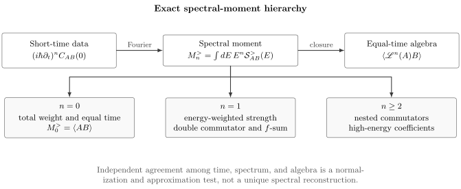
The moment hierarchy can be entered from the time domain, the spectral domain, or equal-time operator algebra. Zeroth moments test normalization, first moments produce energy-weighted identities such as the density $f$-sum, and response moments determine the large-$|z|$ expansion.

The First Three Ordered Moments

Zeroth moment

Completeness gives

$$M_0^{>}[A,B] = \langle AB\rangle.$$

For centered Hermitian $A$,

$$M_0^{>}[A,A] = \langle(\delta A)^2\rangle.$$

This is the total ordered spectral weight. It does not determine whether that weight lies in an elastic line, a sharp mode, several poles, or a continuum.

First moment

The energy-weighted moment is

$$M_1^{>}[A,B] = \langle[A,\mathcal K]B\rangle.$$

For a stationary Hermitian autochannel,

$$\left\langle [A,\mathcal K]A \right\rangle = - \left\langle A[A,\mathcal K] \right\rangle.$$

Therefore

$$M_1^{>}[A,A] = \frac12 \left\langle [A,[\mathcal K,A]] \right\rangle.$$

In a ground state or passive Gibbs state this quantity is nonnegative. A population-inverted stationary state need not obey that positivity.

Second moment

The next moment is

$$M_2^{>}[A,B] = \left\langle [[A,\mathcal K],\mathcal K]B \right\rangle.$$

For Hermitian $A$,

$$M_2^{>}[A,A] = \left\langle [\mathcal K,A][A,\mathcal K] \right\rangle \geq 0.$$

The final expression is the expectation value of

$$[A,\mathcal K]^\dagger [A,\mathcal K].$$

It measures the mean-square energy displacement carried by the operator channel.

Higher moments

Each additional power of $E$ adds one commutator with $\mathcal K$:

$$M_n^{>}[A,B] = \left\langle \mathscr L^n(A)B \right\rangle.$$

The hierarchy can become increasingly nonlocal. For a local Hamiltonian and local $A$, the first few commutators often enlarge the support only by a finite neighborhood. This makes low moments accessible even when the full real-frequency spectrum is difficult to compute.

Response Moments

Define the reversed ordered spectrum

$$\mathcal S_{AB}^{<}(E) := \frac{1}{2\pi\hbar} \int dt\, e^{iEt/\hbar} \langle BA(t)\rangle$$

and the commutator spectral density

$$\rho_{AB}(E) := \mathcal S_{AB}^{>}(E) - \mathcal S_{AB}^{<}(E).$$

Its moments are

$$\begin{aligned} \mu_n[A,B] &:= \int dE\, E^n \rho_{AB}(E) \\ &= \left\langle [ \mathscr L^n(A), B ] \right\rangle. \end{aligned}$$

Because the present retarded convention obeys

$$\chi_{AB}''(E) = \pi\rho_{AB}(E),$$

the same rule is

$$\mu_n[A,B] = \frac{1}{\pi} \int dE\, E^n \chi_{AB}''(E).$$

The first two are

$$\mu_0[A,B] = \langle[A,B]\rangle,$$

and

$$\mu_1[A,B] = \left\langle [[A,\mathcal K],B] \right\rangle.$$

For $B=A$,

$$\mu_1[A,A] = \left\langle [A,[\mathcal K,A]] \right\rangle.$$

This is the double-commutator form used in many energy-weighted response sum rules.

Autochannel parity

For Hermitian $A$,

$$\mathcal S_A^{<}(E) = \mathcal S_A^{>}(-E),$$

so

$$\rho_{AA}(-E) = -\rho_{AA}(E).$$

Consequently,

$$\mu_{2j}[A,A] = 0,$$

while

$$\mu_{2j+1}[A,A] = 2M_{2j+1}^{>}[A,A].$$

For the symmetrized spectrum

$$\mathcal S_A^{\mathrm{sym}}(E) := \frac12 \left[ \mathcal S_A^{>}(E) + \mathcal S_A^{<}(E) \right],$$

all odd moments vanish. Its even moments equal the corresponding even ordered moments.

These parity statements require a Hermitian autochannel. A cross-spectrum or a momentum-resolved pair at fixed $\mathbf q$ can instead relate to the reversed operator order or to $-\mathbf q$.

Thermal form

At Gibbs equilibrium,

$$\mathcal S_{AB}^{<}(E) = e^{-\beta E} \mathcal S_{AB}^{>}(E).$$

Therefore

$$\mu_n[A,B] = \int dE\, E^n \left( 1-e^{-\beta E} \right) \mathcal S_{AB}^{>}(E).$$

This representation exposes the cancellation between thermally forward and reversed transitions. Detailed balance and the moment hierarchy are independent checks: a spectrum can satisfy one and violate the other.

Large-Energy Response

With the source convention

$$H_{\mathrm{pert}}(t) = -f(t)B,$$

the retarded susceptibility has the spectral representation

$$\chi_{AB}(z) = \int_{-\infty}^{\infty} dE'\, \frac{ \rho_{AB}(E') }{ E'-z }.$$

When the necessary moments exist, expand at large complex $z$:

$$\chi_{AB}(z) \sim - \sum_{n=0}^{\infty} \frac{ \mu_n[A,B] }{ z^{n+1} }.$$

Thus

$$\begin{aligned} \chi_{AB}(z) \sim{}& - \frac{ \langle[A,B]\rangle }{z} \\ &- \frac{ \langle[[A,\mathcal K],B]\rangle }{z^2} + \cdots. \end{aligned}$$

For a regular Hermitian autochannel,

$$\begin{aligned} \chi_{AA}(z) \sim{}& - \frac{ \langle[A,[\mathcal K,A]]\rangle }{z^2} \\ &- \frac{ \mu_3[A,A] }{z^4} + \cdots. \end{aligned}$$

The missing odd inverse powers follow from the odd parity of $\rho_{AA}$.

What the expansion tests

The high-energy series tests more than a fitted tail. It simultaneously checks:

• the equal-time operator algebra;
• the generator and chemical-potential convention;
• the normalization of the spectral density;
• the sign of the retarded definition;
• contact or instantaneous terms;
• the asymptotic behavior of a self-energy or approximate propagator.

Matching one coefficient is necessary but not sufficient for causality or conservation.

Contact terms and subtractions

An instantaneous source derivative can add a constant or polynomial term to a response. Such a contact term is not reconstructed from the commutator spectral density alone. Electrical conductivity is the standard example.

If $\chi(z)$ does not decay rapidly enough, use a subtracted dispersion relation or apply the moment expansion to the decaying part. Do not force an unsubtracted sum rule onto a response with a known contact term.

Inverse-Energy-Weighted Moments

Positive moments emphasize high-energy weight. An inverse moment emphasizes the infrared:

$$M_{-1} := \int \frac{dE}{E}\, \rho(E).$$

If there is no singular zero-energy contribution and no subtraction constant,

$$\chi^{\mathrm R}(0) = \int dE\, \frac{\rho(E)}{E}.$$

For a Hermitian autochannel,

$$\chi^{\mathrm R}(0) = 2 \int_0^\infty dE\, \frac{\rho(E)}{E}.$$

Equivalently,

$$\chi^{\mathrm R}(0) = \frac{2}{\pi} \int_0^\infty dE\, \frac{ \chi''(E) }{E}.$$

This is a dynamical static limit. A thermodynamic susceptibility can contain diagonal population rearrangement or conserved-sector contributions that are absent from the strictly isolated retarded limit. The order of $\mathbf q\to0$, $E\to0$, thermodynamic, and relaxation limits must be stated.

An inverse moment can diverge at a gap closing or in a channel with a zero mode. That divergence is physical only after finite-size, elastic, and order-of-limits effects have been separated.

Density f-Sum Rule

Consider $N$ nonrelativistic particles of equal mass $m$ with

$$H = \sum_{j=1}^{N} \frac{\mathbf p_j^2}{2m} + V( \mathbf r_1,\ldots,\mathbf r_N ),$$

where $V$ depends only on positions. Define

$$n_{\mathbf q} := \sum_{j=1}^{N} e^{-i\mathbf q\cdot\mathbf r_j}, \qquad n_{\mathbf q}^\dagger = n_{-\mathbf q}.$$

The potential commutes with every $n_{\mathbf q}$. For the kinetic term,

$$\begin{aligned} [H,n_{-\mathbf q}] ={}& \sum_j e^{i\mathbf q\cdot\mathbf r_j} \\ &\times \left( \frac{\hbar}{m} \mathbf q\cdot\mathbf p_j + \frac{\hbar^2q^2}{2m} \right). \end{aligned}$$

A second commutator removes the momentum-dependent part:

$$\left[ n_{\mathbf q}, [ H,n_{-\mathbf q} ] \right] = \frac{ N\hbar^2q^2 }{m}.$$

Define the per-particle energy-resolved density structure factor by

$$S_n(\mathbf q,E) := \frac{1}{N} \mathcal S_{ n_{\mathbf q}n_{-\mathbf q} }^{>}(E).$$

The exact momentum-symmetrized first moment is

$$\begin{aligned} &\frac12 \int dE\, E \left[ S_n(\mathbf q,E) + S_n(-\mathbf q,E) \right] \\ &\hspace{4em} = \frac{\hbar^2q^2}{2m}. \end{aligned}$$

In equilibrium without directed flow, or whenever the density spectrum is reciprocal under $\mathbf q\to-\mathbf q$,

$$\int dE\, E S_n(\mathbf q,E) = \frac{\hbar^2q^2}{2m}.$$

This is the density $f$-sum rule in the present energy normalization. In angular-frequency normalization,

$$\int d\omega\, \omega S_n(\mathbf q,\omega) = \frac{\hbar q^2}{2m}.$$

Physical interpretation

Interactions can move density spectral weight among a sound mode, a plasmon, multiparticle continua, and high-energy excitations. For position-dependent interactions they cannot change the total energy-weighted density strength. The right-hand side is fixed by mass and canonical kinematics.

The rule does not say that the zeroth moment is interaction independent. It does not say that one mode must exhaust the weight. It does not determine a linewidth. It constrains an integral over the complete spectrum.

Moving states and nonreciprocal media

For one particle in a momentum eigenstate, the transition energy contains a Doppler term proportional to $\mathbf q\cdot\mathbf p$. The moments at $\mathbf q$ and $-\mathbf q$ differ, while their average still gives the recoil energy. This is why the momentum-symmetrized statement is the safest exact form before equilibrium reciprocity is assumed.

Multiple species

For species $a$ with mass $m_a$ and real probe charge or form factor $g_a$, define

$$O_{\mathbf q} := \sum_{a,j} g_a e^{-i\mathbf q\cdot\mathbf r_{aj}}.$$

For local position-dependent interactions, the double commutator gives

$$\frac12 \left\langle [ O_{\mathbf q}, [ H,O_{-\mathbf q} ] ] \right\rangle = \frac{\hbar^2q^2}{2} \sum_a \frac{ N_ag_a^2 }{m_a}.$$

Cross terms do not appear because coordinates of distinct particles commute. Effective low-energy theories can modify this result if degrees of freedom or bands have been projected out.

Lattice and Projected-System Boundary

On a lattice, continuous Galilean kinematics is absent. The first moment is still a double commutator, but its value depends on hopping or band curvature.

For a translationally invariant one-band kinetic Hamiltonian,

$$H_0 = \sum_{\mathbf k,\sigma} \varepsilon_{\mathbf k} c_{\mathbf k\sigma}^\dagger c_{\mathbf k\sigma},$$

the density double commutator contains

$$\begin{aligned} & \left\langle [ n_{\mathbf q}, [ H_0,n_{-\mathbf q} ] ] \right\rangle \\ &= \sum_{\mathbf k,\sigma} \left( \varepsilon_{\mathbf k+\mathbf q} + \varepsilon_{\mathbf k-\mathbf q} - 2\varepsilon_{\mathbf k} \right) \langle n_{\mathbf k\sigma}\rangle. \end{aligned}$$

At small momentum,

$$\begin{aligned} & \varepsilon_{\mathbf k+\mathbf q} + \varepsilon_{\mathbf k-\mathbf q} - 2\varepsilon_{\mathbf k} \\ &= q_\alpha q_\beta \frac{ \partial^2\varepsilon_{\mathbf k} }{ \partial k_\alpha\partial k_\beta } + O(q^4). \end{aligned}$$

The continuum result is recovered only for a quadratic dispersion with the appropriate normalization. Density–density interactions commute with local density, but nonlocal interactions, spin–orbit coupling, multiband geometry, gauge fields, and projected operators can alter the algebra.

Projection changes the rule

Let $P$ project onto a low-energy subspace. In general,

$$P[A,H]P \ne [ PAP, PHP ].$$

Virtual transitions through the discarded space appear on the left but are absent on the right. A projected spectrum should be checked against the projected Hamiltonian and projected operator, with missing interband weight identified explicitly. Comparing it directly to a full-space sum rule can create a false violation.

Optical Sum Preview

The conductivity analogue follows from gauge coupling and includes the diamagnetic contact term. For continuum particles of number density $n$ and electric charge $Q$,

$$\int_0^\infty d\omega\, \operatorname{Re} \sigma_{\alpha\alpha}(\omega) = \frac{ \pi nQ^2 }{ 2m }.$$

The integral includes any zero-frequency delta function with the chosen half-axis convention. Interactions and scattering can redistribute weight between a Drude contribution and finite-frequency absorption without changing the full continuum sum.

On a lattice, the right-hand side is an expectation value of the gauge-curvature or stress operator rather than $nQ^2/m$. The current operator and contact term must be derived from the same gauged Hamiltonian. Kubo Formula develops that source-response structure; Terahertz and Infrared Probes develops experimental partial-weight and superconducting missing-area tests; Transport Coefficients Preview develops the transport limits and coefficient interpretation.

Single-Particle Spectral Moments

For a fermionic spectral matrix $A_{ab}(E)$,

$$\int dE\, A_{ab}(E) = \left\langle \{ c_a,c_b^\dagger \} \right\rangle = \delta_{ab}.$$

Its first moment is

$$\int dE\, E A_{ab}(E) = \left\langle \left\{ [ c_a,\mathcal K ], c_b^\dagger \right\} \right\rangle.$$

The higher hierarchy uses repeated commutators with $\mathcal K$ and the same anticommutator closure. These are graded, number-changing sum rules rather than observable commutator-response rules. Their full Lehmann, occupation, positivity, bosonic, and Nambu conventions remain on Green Functions in Many-Body QM.

Spin and Bond Channels

For a spin component $S_{\mathbf q}^{\alpha}$ in a reciprocal equilibrium state, the energy-weighted structure factor is fixed by

$$\frac12 \left\langle \left[ S_{\mathbf q}^{\alpha}, \left[ H, S_{-\mathbf q}^{\alpha} \right] \right] \right\rangle.$$

Without reciprocity, the displayed double commutator fixes the average of the $\mathbf q$ and $-\mathbf q$ first moments. Unlike the continuum density rule, this expression generally depends on exchange couplings and equal-time bond correlations. The moment can therefore diagnose both normalization and local energetic structure.

For Heisenberg exchange, factors such as

$$1-\cos( \mathbf q\cdot\mathbf r_{ij} )$$

weight the contributing bonds. The small-$\mathbf q$ behavior is controlled by conservation of total spin when the Hamiltonian has the corresponding continuous symmetry. Anisotropy, Dzyaloshinskii–Moriya interactions, fields, and spin–orbit coupling change the commutator.

The same principle applies to bond, nematic, pair, and multipolar channels: define the operator first, then evaluate its commutator with the actual Hamiltonian. Borrowing the density right-hand side for another channel is not valid.

Worked Example: Thermal Harmonic Oscillator

Let

$$H = \hbar\Omega \left( a^\dagger a+\frac12 \right),$$

and

$$X = x_0 \left( a+a^\dagger \right), \qquad x_0 := \sqrt{ \frac{\hbar}{2m\Omega} }.$$

At inverse temperature $\beta$,

$$\bar n = \frac{1}{ e^{\beta\hbar\Omega}-1 }.$$

The ordered spectrum is

$$\begin{aligned} \mathcal S_X^{>}(E) ={}& x_0^2 \left( \bar n+1 \right) \delta( E-\hbar\Omega ) \\ &+ x_0^2 \bar n \delta( E+\hbar\Omega ). \end{aligned}$$

Its first three moments are

$$M_0^{>} = x_0^2 \left( 2\bar n+1 \right),$$ $$M_1^{>} = x_0^2 \hbar\Omega = \frac{\hbar^2}{2m},$$

and

$$M_2^{>} = x_0^2 (\hbar\Omega)^2 \left( 2\bar n+1 \right).$$

The zeroth and second moments grow with temperature. The first moment does not, because thermal upward and downward contributions cancel all occupation dependence.

Directly,

$$[X,[H,X]] = \frac{\hbar^2}{m},$$

so

$$M_1^{>} = \frac12 \langle[X,[H,X]]\rangle = \frac{\hbar^2}{2m}.$$

The example also shows why discarding the negative-energy thermal line breaks an exact full-spectrum moment.

Worked Example: A Spin Dimer

Take two dimensionless spin-$1/2$ operators,

$$H = J\, \mathbf s_1\cdot\mathbf s_2, \qquad J\gt0,$$

and the staggered detector

$$A := s_1^z-s_2^z.$$

The ground state is the singlet $\lvert s\rangle$, and

$$A\lvert s\rangle = \lvert t_0\rangle.$$

The singlet-to-triplet gap is $J$, so

$$\mathcal S_A^{>}(E) = \delta(E-J).$$

Therefore

$$M_0^{>}=1, \qquad M_1^{>}=J.$$

The double commutator gives

$$\frac12 \langle s| [A,[H,A]] |s\rangle = J.$$

Here one line exhausts the zeroth and first moments. In an extended interacting magnet, the same weight can be shared among magnons, bound states, and continua while the exact moment remains fixed.

Moment Inequalities

For a Hermitian ordered spectrum, $\mathcal S_A^{>}(E)$ is a nonnegative measure. Hence every squared polynomial has nonnegative average:

$$\int dE\, \left| \sum_{j=0}^{r} v_jE^j \right|^2 \mathcal S_A^{>}(E) \geq 0.$$

The Hankel moment matrix

$$\mathsf H_{ij} := M_{i+j}^{>}, \qquad i,j=0,\ldots,r,$$

must therefore be positive semidefinite. The first nontrivial condition is

$$M_0^{>}M_2^{>} - \left( M_1^{>} \right)^2 \geq 0.$$

If $M_0^{>}\ne0$, define the spectral centroid and variance:

$$\bar E := \frac{M_1^{>}}{M_0^{>}},$$ $$\operatorname{Var}(E) := \frac{M_2^{>}}{M_0^{>}} - \bar E^2 \geq 0.$$

The centroid is not automatically a quasiparticle energy. The variance is not automatically an intrinsic linewidth. Both include all poles and continua in the chosen operator channel.

Support bounds

Suppose a zero-temperature inelastic spectrum has support only for

$$E\geq\Delta\gt0.$$

Then

$$M_1^{>} \geq \Delta M_0^{>},$$

so

$$\Delta \leq \frac{M_1^{>}}{M_0^{>}}.$$

The ratio gives an upper bound on the lowest visible excitation energy, not a lower bound. Equality requires all visible weight to lie at one energy.

If $E\geq0$ and a higher moment $M_p^{>}$ is known, the weight above a cutoff $E_c$ obeys

$$\int_{E_c}^{\infty} dE\, \mathcal S_A^{>}(E) \leq \frac{ M_p^{>} }{ E_c^p }.$$

This bound can quantify how much unmeasured high-energy weight is compatible with a known moment.

Partial and Windowed Moments

An experiment or numerical reconstruction usually provides

$$M_n^{[E_-,E_+]} := \int_{E_-}^{E_+} dE\, E^n \mathcal S(E),$$

not the full moment. A partial moment is useful, but it is not the exact sum rule unless all omitted contributions are shown to vanish or are bounded.

Missing contributions can include:

• an elastic line;
• thermally reversed negative-energy weight;
• a high-energy continuum;
• another band or particle-number sector;
• a symmetry-related momentum channel;
• tails outside the detector window;
• probe matrix elements and polarization factors;
• background subtraction that removed genuine signal.

Every reported saturation fraction should specify the operator, normalization, integration measure, energy window, elastic convention, and estimated missing weight.

Resolution and Artificial Broadening

Let a measured spectrum be a convolution

$$\mathcal S_{\mathrm{obs}}(E) = \int dE'\, R(E-E') \mathcal S(E'),$$

with normalized kernel

$$\int d\epsilon\, R(\epsilon) = 1.$$

Define kernel moments

$$r_j := \int d\epsilon\, \epsilon^j R(\epsilon).$$

Then

$$M_0^{\mathrm{obs}} = M_0,$$ $$M_1^{\mathrm{obs}} = M_1+r_1M_0,$$

and

$$M_2^{\mathrm{obs}} = M_2 + 2r_1M_1 + r_2M_0.$$

A centered Gaussian resolution has $r_1=0$ and preserves the first moment, but it increases the second moment by its variance times $M_0$.

A Lorentzian has heavy tails. Although its zeroth moment is normalized, its ordinary first absolute moment and second moment diverge on an infinite domain. Replacing every delta line by a Lorentzian can therefore destroy higher moment tests even when the underlying discrete spectrum satisfies them exactly.

Finite-window integration of the broadened curve adds a separate boundary error. Broadening, truncation, and physical decay must be tracked independently.

Numerical Validation

Independent sides of the identity

A meaningful check computes the two sides independently:

1. Integrate or sum the spectral representation.
2. Evaluate the equal-time product or nested commutator directly.
3. Compare them using the same state, generator, operator normalization, and finite-size geometry.

If both sides are generated from the same already-truncated spectral list, agreement can be tautological.

Exact diagonalization

For exact diagonalization, include:

• every symmetry sector reached by the operator;
• all degenerate states and thermal weights;
• continuum substitutes or basis-cutoff effects;
• bin widths and delta-function normalization;
• negative-energy thermal transitions;
• the same broadening convention on both sides only when appropriate.

Low moments can converge slowly because powers of energy amplify weak high-energy weight. Apparent convergence of a low-energy peak does not establish convergence of the $f$-sum.

Krylov and continued-fraction methods

A Krylov space generated from

$$A\lvert\Psi\rangle$$

is naturally adapted to moments. The Lanczos recursion encodes low-order powers of $H$ and can reproduce a corresponding set of moments before resolving every spectral feature. Lanczos Method Preview derives the tridiagonal response representation and its finite-system evidence ledger. Loss of orthogonality, termination, finite precision, and thermal sampling still require checks.

Imaginary-time and analytic continuation

Imaginary-time data constrain weighted integrals of the real-frequency spectrum. Exact moments can regularize continuation and reject impossible spectra, but finitely many moments do not make the inverse problem unique.

A continuation workflow should test:

• positivity only in channels where it is valid;
• exact zeroth and known higher moments;
• covariance-aware agreement with imaginary-time data;
• sensitivity to the prior or regularizer;
• synthetic spectra with hidden high-energy weight;
• stability when moment constraints are relaxed within uncertainty.

Imposing an incorrect moment exactly can make a reconstruction look stable while biasing every feature.

Time-domain data

Moments can be estimated from derivatives at $t=0$, but numerical differentiation amplifies noise. A finite time step, asymmetric stencil, or nonanalytic short-time cusp can dominate high derivatives.

Compare derivative estimates to direct commutators whenever possible. Long-time data determine fine spectral resolution; short-time data determine broad moments. These are complementary constraints.

Approximation Diagnostics

For an approximate spectrum, define a residual

$$\Delta_n := M_n^{\mathrm{spec}} - M_n^{\mathrm{alg}},$$

where the second term is evaluated from the approximation’s stated Hamiltonian, state, and operator algebra. A dimensionless residual can use

$$\varepsilon_n := \frac{ \lvert\Delta_n\rvert }{ \lvert M_n^{\mathrm{spec}}\rvert + \lvert M_n^{\mathrm{alg}}\rvert + s_n },$$

with a declared numerical floor $s_n$.

Near a symmetry-forced zero, an absolute tolerance is more informative than a relative one.

Necessary, not sufficient

Passing several sum rules does not prove that:

• the line shape is correct;
• causality holds;
• detailed balance holds;
• a Ward identity is satisfied;
• the approximation is conserving;
• the thermodynamic limit is controlled;
• an analytic continuation is unique.

It only proves agreement with the tested integrated constraints.

Conserving approximations

Conservation laws link vertices, self-energies, currents, and contact terms. An approximation can have a causal propagator yet violate a density or optical sum rule because its vertex is inconsistent. Conversely, a fitted spectrum can be normalized to one moment while violating the underlying continuity equation.

Check conservation laws, Ward identities, positivity, KMS balance, and moments as distinct conditions.

Truncation and Canonical Algebra

No finite-dimensional matrices can satisfy

$$[X,P] = i\hbar I$$

exactly, because the trace of a finite-dimensional commutator vanishes while

$$\operatorname{Tr}(i\hbar I) \ne 0.$$

A truncated oscillator basis therefore develops boundary defects in canonical commutators. Low-lying states may satisfy position sum rules accurately while states near the cutoff fail badly.

The correct diagnostic is not to demand impossible full-space algebra from finite matrices. Instead:

1. identify the projected operator and Hamiltonian;
2. evaluate the projected commutator;
3. monitor boundary-state occupation;
4. increase the cutoff;
5. test convergence for the states and moments of interest.

The same issue appears in truncated bosonic occupations, finite plane-wave bases, pseudopotentials, and low-band effective models.

Experimental Use

To compare a measured spectrum with an exact sum rule:

1. Identify the intrinsic operator correlator behind the cross section.
2. Remove or model form factors, polarization projectors, kinematic factors, and detector efficiency.
3. State whether the elastic line is included.
4. Include both energy-transfer directions when temperature makes them relevant.
5. Convert counts to the same absolute normalization as the equal-time expectation value.
6. Integrate over a declared energy and momentum region.
7. Propagate background and resolution uncertainty into the moment.
8. Estimate unmeasured tails using theory, auxiliary data, or moment bounds.
9. Compare several moments rather than only total area.

Agreement after an arbitrary vertical rescaling is not a test of an absolute sum rule.

Common Mistakes

• Mixing energy and angular-frequency moments without the required powers of $\hbar$.
• Using $H$ in the spectrum and $H-\mu\hat N$ in the commutator for a number-changing operator.
• Forgetting the negative-energy thermal branch.
• Applying autochannel parity to a cross-channel or fixed nonreciprocal momentum.
• Treating a partial-window integral as the full sum.
• Omitting elastic, Drude, interband, or continuum weight.
• Using the continuum density right-hand side for a lattice or projected model.
• Dropping contact terms from conductivity.
• Assuming normalized broadening preserves every moment.
• Interpreting $M_1/M_0$ as a unique mode energy when a continuum is present.
• Applying positivity inequalities to a signed commutator spectrum.
• Ignoring unbounded-operator domains or ultraviolet divergences.
• Comparing a full-space algebraic rule to a truncated-space spectrum.
• Declaring an approximation correct because one moment was imposed by hand.

Reliable Workflow

1. Define the operator channel and whether it is centered.
2. Declare the stationary state and evolution generator.
3. Fix energy or angular-frequency normalization.
4. Write the Lehmann representation and identify positivity or sign structure.
5. Choose ordered, symmetrized, or commutator moments.
6. Verify that the desired moment exists.
7. Evaluate the nested commutator independently.
8. Include momentum reversal, contact terms, and projected-space corrections where required.
9. Separate full, partial, elastic, and broadened moments.
10. Quantify numerical, cutoff, resolution, and tail errors.
11. Check several independent constraints.
12. Interpret the result only within the operator channel and measured window.

Exercises

Exercise 1: Derive the master hierarchy

Starting from

$$\langle A(t)B\rangle = \int dE\, e^{-iEt/\hbar} \mathcal S_{AB}^{>}(E),$$

derive

$$\int dE\, E^n \mathcal S_{AB}^{>}(E) = \langle\mathscr L^n(A)B\rangle.$$

Solution

Apply $(i\hbar\partial_t)^n$ to the inverse transform:

$$\begin{aligned} &(i\hbar\partial_t)^n \langle A(t)B\rangle \\ &= \int dE\, E^n e^{-iEt/\hbar} \mathcal S_{AB}^{>}(E). \end{aligned}$$

At $t=0$, the right-hand side is the $n$th moment. Heisenberg evolution gives

$$i\hbar \frac{dA(t)}{dt} = [A(t),\mathcal K] = \mathscr L(A(t)).$$

Repeated differentiation therefore gives

$$\left. (i\hbar\partial_t)^n A(t) \right|_{t=0} = \mathscr L^n(A).$$

Combining the two equations proves the result.

Exercise 2: Autochannel parity

For Hermitian $A$, prove that the commutator spectrum is odd and show that

$$\mu_1[A,A] = 2M_1^{>}[A,A] = \langle[A,[\mathcal K,A]]\rangle.$$

Solution

Interchanging the two Lehmann labels gives

$$\mathcal S_A^{<}(E) = \mathcal S_A^{>}(-E).$$

Hence

$$\begin{aligned} \rho_{AA}(-E) &= \mathcal S_A^{>}(-E) - \mathcal S_A^{<}(-E) \\ &= \mathcal S_A^{<}(E) - \mathcal S_A^{>}(E) \\ &= -\rho_{AA}(E). \end{aligned}$$

For the first moment,

$$\begin{aligned} \mu_1 &= \int dE\, E \left[ \mathcal S_A^{>}(E) - \mathcal S_A^{>}(-E) \right] \\ &= 2 \int dE\, E \mathcal S_A^{>}(E) \\ &= 2M_1^{>}. \end{aligned}$$

The response moment theorem gives

$$\mu_1 = \langle[[A,\mathcal K],A]\rangle = \langle[A,[\mathcal K,A]]\rangle.$$

Exercise 3: Thermal oscillator moments

Use

$$\begin{aligned} \mathcal S_X^{>}(E) ={}& x_0^2 (\bar n+1) \delta(E-\hbar\Omega) \\ &+ x_0^2 \bar n \delta(E+\hbar\Omega) \end{aligned}$$

to compute $M_0^{>}$, $M_1^{>}$, and $M_2^{>}$. Explain why the odd first moment is temperature independent while the even zeroth and second moments are not.

Solution

Direct integration gives

$$M_0^{>} = x_0^2 \left( 2\bar n+1 \right).$$

For the first moment,

$$\begin{aligned} M_1^{>} &= x_0^2 \hbar\Omega \left[ (\bar n+1)-\bar n \right] \\ &= x_0^2\hbar\Omega \\ &= \frac{\hbar^2}{2m}. \end{aligned}$$

For the second,

$$M_2^{>} = x_0^2 (\hbar\Omega)^2 \left( 2\bar n+1 \right).$$

Odd powers assign opposite signs to the two thermal branches, so detailed-balance occupations cancel in $M_1^{>}$. Even powers add them.

Exercise 4: Continuum density f-sum

For one particle, prove

$$\left[ e^{-i\mathbf q\cdot\mathbf r}, \left[ \frac{\mathbf p^2}{2m}, e^{i\mathbf q\cdot\mathbf r} \right] \right] = \frac{\hbar^2q^2}{m}.$$

Extend the result to $N$ particles with position-dependent interactions.

Solution

Use

$$\mathbf p\, e^{i\mathbf q\cdot\mathbf r} = e^{i\mathbf q\cdot\mathbf r} \left( \mathbf p+\hbar\mathbf q \right).$$

Then

$$\begin{aligned} \left[ \frac{\mathbf p^2}{2m}, e^{i\mathbf q\cdot\mathbf r} \right] ={}& e^{i\mathbf q\cdot\mathbf r} \\ &\times \left( \frac{\hbar}{m} \mathbf q\cdot\mathbf p + \frac{\hbar^2q^2}{2m} \right). \end{aligned}$$

Commuting $e^{-i\mathbf q\cdot\mathbf r}$ through the remaining momentum shifts it by $-\hbar\mathbf q$, leaving

$$\frac{\hbar^2q^2}{m}.$$

Terms associated with different particles commute. A position-dependent interaction also commutes with every density phase. Summing the one-particle result gives

$$\left[ n_{\mathbf q}, [H,n_{-\mathbf q}] \right] = \frac{N\hbar^2q^2}{m}.$$

Half of this response moment gives the reciprocal equilibrium ordered first moment.

Exercise 5: Lattice curvature

Let

$$\varepsilon_k = -2t\cos(ka)$$

in one dimension. Evaluate

$$\varepsilon_{k+q} + \varepsilon_{k-q} - 2\varepsilon_k$$

and find its leading small-$q$ form.

Solution

Using

$$\begin{aligned} & \cos\left((k+q)a\right) + \cos\left((k-q)a\right) \\ &\qquad = 2\cos(ka)\cos(qa), \end{aligned}$$

one obtains

$$\begin{aligned} & \varepsilon_{k+q} + \varepsilon_{k-q} - 2\varepsilon_k \\ &= 4t\cos(ka) \left[ 1-\cos(qa) \right]. \end{aligned}$$

For small $q$,

$$1-\cos(qa) = \frac{q^2a^2}{2} + O(q^4),$$

so

$$\begin{aligned} & \varepsilon_{k+q} + \varepsilon_{k-q} - 2\varepsilon_k \\ &\qquad = 2ta^2q^2 \cos(ka) + O(q^4). \end{aligned}$$

The coefficient depends on the occupied-band curvature. It is not the universal continuum value $\hbar^2q^2/m$ unless the dispersion is approximated by a quadratic band with a specified effective mass.

Exercise 6: Centroid and width inequality

Use positivity to prove

$$\left( M_1^{>} \right)^2 \leq M_0^{>}M_2^{>}.$$

When does equality hold?

Solution

Apply Cauchy–Schwarz in the measure

$$d\mu(E) := \mathcal S_A^{>}(E)dE$$

to the functions $1$ and $E$:

$$\left| \int d\mu\,E \right|^2 \leq \left( \int d\mu \right) \left( \int d\mu\,E^2 \right).$$

This is

$$\left( M_1^{>} \right)^2 \leq M_0^{>}M_2^{>}.$$

Equality in Cauchy–Schwarz requires $E$ to be constant almost everywhere with respect to the spectral measure. Thus all nonzero spectral weight must lie at one energy.

Exercise 7: Resolution moments

Suppose $R$ is normalized, centered, and has variance $\sigma_R^2$. Show that convolution preserves $M_0$ and $M_1$ but changes $M_2$.

Solution

Write $E=E'+\epsilon$ in the convolution integral. Normalization gives

$$M_0^{\mathrm{obs}} = M_0.$$

Centering means

$$\int d\epsilon\, \epsilon R(\epsilon) = 0,$$

so

$$M_1^{\mathrm{obs}} = M_1.$$

For the second moment,

$$(E'+\epsilon)^2 = E'^2 + 2E'\epsilon + \epsilon^2.$$

The cross term vanishes after averaging over a centered kernel, leaving

$$M_2^{\mathrm{obs}} = M_2 + \sigma_R^2M_0.$$

Instrumental broadening therefore contributes to a measured spectral variance even when it preserves total area and centroid.

Exercise 8: Missing high-energy weight

A nonnegative zero-temperature spectrum has known $M_0$ and $M_2$. Derive an upper bound on the total weight above $E_c\gt0$. Explain what the bound cannot determine.

Solution

For $E\geq E_c$,

$$1 \leq \frac{E^2}{E_c^2}.$$

Multiplying by the nonnegative spectrum and integrating gives

$$\begin{aligned} \int_{E_c}^{\infty} dE\, \mathcal S(E) &\leq \frac{1}{E_c^2} \int_{E_c}^{\infty} dE\, E^2\mathcal S(E) \\ &\leq \frac{M_2}{E_c^2}. \end{aligned}$$

The bound limits the total missing weight. It does not locate that weight, determine its line shape, or prove that the bound is saturated.

Cross-Links

• Linear Response Formula Sheet: compact spectral, dispersion, contact-term, and limit-order conventions.
• Time-Dependent Correlations: Lehmann spectra and short-time versus long-time information.
• Structure Factors: density and spin normalization, scattering, and the single-mode relation.
• Green Functions in Many-Body QM: canonical single-particle spectral moments.
• Retarded and Advanced Response: spectral representations and dispersion relations.
• Kubo Formula: source derivatives, contact terms, and conductivity.
• Transport Coefficients Preview: conductivity, diffusion, viscosity, and hydrodynamic limit order.
• Fluctuation–Dissipation Theorem: detailed balance and absorptive response.
• Spectral Functions: peaks, continua, linewidths, and forward models.
• Lanczos Method Preview: Krylov moment matching, continued fractions, and solver diagnostics.
• Sum Rules and Completeness Tricks: closure methods and state-by-state oscillator-strength identities.
• Commutators: algebraic identities used in nested-commutator calculations.

References

1. R. Kubo, “Statistical-Mechanical Theory of Irreversible Processes. I”, Journal of the Physical Society of Japan 12, 570–586 (1957).
2. P. C. Hohenberg and W. F. Brinkman, “Sum Rules for the Frequency Spectrum of Linear Magnetic Chains”, Physical Review B 10, 128–131 (1974).
3. R. P. Feynman, “Atomic Theory of the Two-Fluid Model of Liquid Helium”, Physical Review 94, 262–277 (1954).
4. A. L. Fetter and J. D. Walecka, Quantum Theory of Many-Particle Systems, Dover (2003).
5. P. Nozières and D. Pines, The Theory of Quantum Liquids, Westview Press (1999).
6. G. D. Mahan, Many-Particle Physics, 3rd ed., Springer (2000).
7. D. Forster, Hydrodynamic Fluctuations, Broken Symmetry, and Correlation Functions, CRC Press (1990).
8. G. L. Squires, Introduction to the Theory of Thermal Neutron Scattering, 3rd ed., Cambridge University Press (2012).
9. W. Kohn, “Theory of the Insulating State”, Physical Review 133, A171–A181 (1964).