Plasmons Preview

A plasmon is a quantum of a collective charge-density oscillation. Mobile charges move coherently, create an electric field, and are driven back by that self-consistent field. When the resulting branch is sufficiently underdamped, one can quantize it and speak of individual plasmons.

In a three-dimensional homogeneous electron fluid, the long-range Coulomb interaction changes the infrared behavior qualitatively:

$$\lim_{q\to0}\omega_{\mathrm{pl}}(q) = \omega_{\mathrm p} \ne0.$$

The simplest SI plasma frequency is

$$\omega_{\mathrm p}^2 = \frac{n_0Q^2} {m\epsilon_0\epsilon_{\mathrm b}},$$

where $n_0$ is carrier number density, $Q$ is carrier charge, $m$ is the inertial mass, and $\epsilon_{\mathrm b}$ is a dimensionless background dielectric constant.

This finite frequency is not universal across geometry. A two-dimensional sheet coupled through three-dimensional electric fields has

$$\omega_{\mathrm{pl}}(q)\propto\sqrt q,$$

while a nearby metallic gate can make the longest-wavelength branch acoustic. Dimension, dielectric environment, boundaries, screening, band structure, and other mobile species are part of the definition of the problem.

Scope and Canonical Ownership

This page owns the general physical framework:

• why long-range Coulomb forces reorganize density motion into collective charge modes;
• the hydrodynamic derivation and interpretation of the bulk plasma frequency;
• the exact distinction between $q=0$ and the limit $q\to0$;
• dimensional scaling from the Coulomb kernel;
• dielectric zeros, screened-response poles, and loss peaks;
• the distinction among density response, structure factor, conductivity, and loss function;
• complex mode frequency, quality factor, and Landau damping;
• spectral weight and the density $f$-sum rule;
• bulk, sheet, gated, surface, and electromagnetic mode taxonomy at preview level;
• coupling to phonons, charged-superfluid phase modes, and multiple carrier species;
• experimental diagnostics and practical identification criteria.

Neighboring pages retain their canonical subjects:

• Random Phase Approximation owns the Lindhard function, bubble resummation, dielectric denominator, explicit RPA plasmon derivation, and RPA validity analysis.
• Density Operators and Current Operators owns microscopic density, current, and continuity-equation conventions.
• Susceptibilities owns source signs, response units, order of limits, and static thermodynamic susceptibilities.
• Particle–Hole Excitations owns continuum kinematics and Pauli-blocked phase space.
• Structure Factors owns exact scattering-spectrum normalization and experimental vertices.
• Sum Rules owns the nested-commutator derivation and complete moment hierarchy.
• Collective Modes owns the general response-eigenmode, hybridization, and damping language.
• Goldstone Modes in Many-Body Systems owns the charged-superfluid Anderson–Higgs interpretation.

Detailed band- and material-specific plasmons, surface plasmonics, nanostructure modes, first-principles dielectric calculations, and device applications route through the Lattice Vibrations and Collective Modes gateway to their material, electromagnetic-boundary, computational, and probe owners. The present page supplies the reusable many-body principles without duplicating that materials treatment.

Convention Ledger

Frequency and energy

The mode variable $\omega$ is angular frequency. The corresponding quantum energy is

$$E_{\mathrm{pl}}(\mathbf q) = \hbar\omega_{\mathrm{pl}}(\mathbf q).$$

Plasma frequency and plasma energy must not be quoted with the same units.

Charge and density

The carrier charge $Q$ is signed. For electrons, $Q=-e$. The restoring scale depends on

$$Q^2=e^2,$$

so the bulk frequency is positive regardless of the sign convention. Number- and charge-density fluctuations are related by

$$\delta\rho(\mathbf r,t) = Q\,\delta n(\mathbf r,t).$$

The uniform equilibrium background is neutral:

$$\rho_{\mathrm{back}} +Qn_0=0.$$

Without this background or an explicit boundary-value prescription, the Coulomb energy of a uniformly charged infinite system is undefined.

Fourier convention

Plane waves vary as

$$e^{i(\mathbf q\cdot\mathbf r-\omega t)}.$$

The wave vector is $\mathbf q$ and the physical momentum transferred by one plasmon is $\hbar\mathbf q$.

For a three-dimensional SI Coulomb interaction screened by a background dielectric,

$$v_{\mathbf q}^{3\mathrm D} = \frac{Q^2} {\epsilon_0\epsilon_{\mathrm b}q^2}.$$

This is the Fourier coefficient of interaction energy in the convention

$$V(r) = \frac{Q^2} {4\pi\epsilon_0\epsilon_{\mathrm b}r}.$$

In Gaussian units the corresponding formulas are

$$v_{\mathbf q}^{3\mathrm D} = \frac{4\pi Q^2}{\epsilon_{\mathrm b}q^2}, \qquad \omega_{\mathrm p}^2 = \frac{4\pi n_0Q^2}{m\epsilon_{\mathrm b}}.$$

The factor $4\pi$ moves with the electromagnetic unit system; it is not a physical disagreement.

Polarization sign

Let a potential energy $U_{\mathrm{ext}}$ couple to number density:

$$\delta K_{\mathrm{ext}} = \int d^dr\, U_{\mathrm{ext}}(\mathbf r,t)n(\mathbf r).$$

Define the retarded polarization by

$$\delta n(\mathbf q,\omega) = \Pi^R(\mathbf q,\omega) U_{\mathrm{ext}}(\mathbf q,\omega).$$

A positive static potential energy repels particles, so

$$\Pi^R(q\to0,0)<0.$$

The chemical-potential susceptibility used elsewhere obeys

$$\chi_{nn}^R=-\Pi^R.$$

This page follows the polarization sign because it gives the familiar dielectric denominator $1-v\Pi$.

Background-normalized dielectric function

The Coulomb kernel already contains $\epsilon_{\mathrm b}$. It is therefore convenient to define

$$\bar\epsilon_L(\mathbf q,\omega) := \frac{\epsilon_L^{\mathrm{phys}}(\mathbf q,\omega)} {\epsilon_{\mathrm b}}.$$

In a scalar homogeneous channel,

$$\bar\epsilon_L = 1-v_{\mathbf q}P^R,$$

where $P^R$ is the density polarization irreducible with respect to one Coulomb line. Multiplying by the nonzero constant $\epsilon_{\mathrm b}$ does not change dielectric zeros, but it does rescale a quoted loss function.

What Makes a Mode a Plasmon

Collective charge motion

A plasmon is not one electron promoted to another orbital. In a finite basis, one plasmon state is a coherent superposition of many particle–hole configurations:

$$|\mathrm{pl},\mathbf q\rangle \sim \sum_{\mathbf k,\sigma} X_{\mathbf k\mathbf q} c_{\mathbf k+\mathbf q,\sigma}^\dagger c_{\mathbf k\sigma} |\mathrm{FS}\rangle +\cdots.$$

The coefficients align the microscopic transitions so their induced electric fields reinforce one another. The omitted terms can contain backward amplitudes, multiple pairs, interband transitions, and correlation corrections.

Longitudinal character

In the electrostatic bulk limit, the charge-density wave and electric field are longitudinal:

$$\mathbf E_L \parallel \mathbf q.$$

Gauss’s law ties the longitudinal field directly to charge density. A transverse electromagnetic wave instead satisfies a Maxwell dispersion relation and can hybridize with matter to form a polariton. The words plasmon and plasmon polariton should not be used interchangeably without stating the geometry and retardation regime.

One plasmon is a bosonic quantum

After linearization and normal-mode diagonalization, a sharp branch has an effective harmonic Hamiltonian

$$H_{\mathrm{pl}} = \sum_{\mathbf q} \hbar\omega_{\mathrm{pl}}(\mathbf q) \left( b_{\mathbf q}^\dagger b_{\mathbf q} +\frac12 \right).$$

The operators $b_{\mathbf q}$ are bosonic within the dilute-excitation harmonic description. This algebra comes from quantizing a collective coordinate, not from the microscopic electrons being bosons.

When damping is strong, no unique Hermitian oscillator mode may exist. One then has a charge-density resonance or continuum rather than a long-lived plasmon quasiparticle.

Hydrodynamic Bulk Derivation

Linearized continuity equation

Let the carrier fluid have equilibrium density $n_0$, fluctuation $\delta n$, and velocity $\mathbf u$. Number conservation gives

$$\partial_t\delta n + n_0\nabla\cdot\mathbf u =0.$$

For a plane wave,

$$-i\omega\,\delta n + in_0\mathbf q\cdot\mathbf u =0.$$

Only the longitudinal velocity contributes to a density fluctuation.

Force balance

The linearized inertial equation is

$$m\partial_t\mathbf u = Q\mathbf E - \frac1{n_0}\nabla\delta P.$$

The pressure term summarizes the restoring force that would produce neutral sound. For the charge fluctuation, Gauss’s law is

$$\nabla\cdot\mathbf E = \frac{Q\,\delta n} {\epsilon_0\epsilon_{\mathrm b}}.$$

Differentiate the continuity equation in time and insert force balance:

$$\partial_t^2\delta n = -\frac{n_0Q^2} {m\epsilon_0\epsilon_{\mathrm b}} \delta n + \frac1m\nabla^2\delta P.$$

If the dynamic pressure closure is

$$\delta P = \left( \frac{\partial P}{\partial n} \right)_{\mathrm{dyn}} \delta n,$$

define

$$c_{\mathrm{dyn}}^2 := \frac1m \left( \frac{\partial P}{\partial n} \right)_{\mathrm{dyn}}.$$

The dispersion is

$$\omega^2(q) = \omega_{\mathrm p}^2 + c_{\mathrm{dyn}}^2q^2,$$

with

$$\omega_{\mathrm p}^2 = \frac{n_0Q^2} {m\epsilon_0\epsilon_{\mathrm b}}.$$

Physical interpretation

For a neutral compressional wave, the restoring force decreases with wavelength because it comes from gradients of pressure. Its frequency is acoustic:

$$\omega_{\mathrm{neutral}}\sim cq.$$

For a charged wave in three dimensions, the Coulomb kernel grows as $q^{-2}$. The density modulation shrinks at long wavelength, but its electric potential becomes longer ranged. The two powers cancel, leaving a finite frequency.

The pressure coefficient beyond the leading gap is regime-dependent. In a collisionless three-dimensional ideal Fermi gas, long-wavelength RPA gives a $q^2$ coefficient proportional to $3v_F^2/5$. A hydrodynamic thermodynamic closure gives a different coefficient. Both can share the same leading $\omega_{\mathrm p}$ while describing different orderings of collision rate, frequency, and wavelength.

Inertial mass

The mass in the continuum formula is the mass controlling longitudinal current response. It is the bare carrier mass in a Galilean-invariant parabolic continuum. In a crystal it is replaced by band and interaction-dependent Drude-weight data, often tensorial.

Writing

$$\omega_{\mathrm p}^2 = \frac{ne^2}{m_e\epsilon_0}$$

for every metal silently discards background screening, band structure, multiple carriers, and anisotropy.

Exactly Zero Momentum Versus the Limit

Conserved uniform density

The Fourier density at exactly zero wave vector is the total particle number:

$$n_{\mathbf q=0}=N.$$

For a closed number-conserving system,

$$[H,N]=0.$$

Therefore the exactly uniform density operator cannot create a finite-frequency excitation in the fixed-$N$ sector.

The nonuniform limiting sequence

A bulk plasmon is defined by a sequence of nonzero wave vectors:

$$\omega_{\mathrm p} = \lim_{q\to0^+} \omega_{\mathrm{pl}}(q).$$

Every member of the sequence has positive and negative charge regions and preserves total charge:

$$\int d^dr\,\delta\rho_{\mathbf q}(\mathbf r)=0 \qquad (\mathbf q\ne0).$$

There is no contradiction between a conserved $q=0$ density and a finite limiting frequency at $q\to0$.

Oscillator strength vanishes appropriately

Although the frequency stays finite in three dimensions, the density matrix element vanishes with $q$. If one mode exhausts the long-wavelength density $f$-sum rule,

$$\frac1N \left| \langle\mathrm{pl},\mathbf q| n_{\mathbf q}|0\rangle \right|^2 \simeq \frac{\hbar q^2} {2m\omega_{\mathrm p}}.$$

Thus the density weight is proportional to $q^2$. Number conservation is respected even while the mode energy tends to $\hbar\omega_{\mathrm p}$.

Long-Range Forces Set the Infrared Scaling

General small-wave-vector estimate

Continuity and longitudinal inertia imply the high-frequency, small-$q$ polarization of a parabolic carrier fluid:

$$P^R(q,\omega) \simeq \frac{n_dq^2} {m(\omega+i0^+)^2}.$$

Here $n_d$ is a density appropriate to the carrier dimension. Combining this with

$$\bar\epsilon_L(q,\omega) = 1-v_qP^R(q,\omega)$$

gives the leading collective scale

$$\omega_{\mathrm{pl}}^2(q) \simeq \frac{n_dq^2v_q}{m}.$$

This one relation explains why the same charge carriers can have gapped, square-root, nearly acoustic, or acoustic plasmons in different geometries.

Three-dimensional bulk

For

$$v_q^{3\mathrm D} = \frac{Q^2} {\epsilon_0\epsilon_{\mathrm b}q^2},$$

the factors of $q^2$ cancel:

$$\omega_{\mathrm{pl}}^2(q\to0) = \frac{n_3Q^2} {m\epsilon_0\epsilon_{\mathrm b}}.$$

The mode is gapped in the long-wavelength sense even though the metal has no one-particle excitation gap at its Fermi surface.

Two-dimensional sheet

For carriers confined to a sheet while electric fields occupy three-dimensional space,

$$v_q^{2\mathrm D} = \frac{Q^2} {2\epsilon_0\epsilon_{\mathrm{eff}}q}.$$

Then

$$\omega_{\mathrm{pl}}^2(q) \simeq \frac{ n_2Q^2 }{2m\epsilon_0\epsilon_{\mathrm{eff}}} q,$$

and therefore

$$\omega_{\mathrm{pl}}(q)\propto\sqrt q.$$

The density $n_2$ is an areal density. Substituting a volume density into this formula is dimensionally wrong.

Quasi-one-dimensional wire

For a thin isolated wire of transverse scale $a$, the effective Coulomb kernel behaves schematically as

$$v_q^{1\mathrm D} \propto \left|\ln(qa)\right|$$

at small $qa$. The collective branch then scales as

$$\omega_{\mathrm{pl}}(q) \propto q\sqrt{|\ln(qa)|}.$$

The logarithm and its constant depend on the transverse charge profile and dielectric boundaries. A strictly one-dimensional $1/|x|$ model requires an ultraviolet prescription.

Short-range or gate-screened interaction

If the effective interaction approaches a constant,

$$v_q\to v_0,$$

then

$$\omega_{\mathrm{coll}}(q) \simeq q\sqrt{\frac{n_dv_0}{m}}.$$

The branch is acoustic. Long-range Coulomb interaction is what distinguishes the bulk three-dimensional plasma gap from neutral sound.

Geometry table

Carrier geometry	Small-$q$ interaction	Leading branch
3D bulk	$v_q\propto q^{-2}$	$\omega_{\mathrm{pl}}\to\omega_{\mathrm p}$
isolated 2D sheet	$v_q\propto q^{-1}$	$\omega_{\mathrm{pl}}\propto q^{1/2}$
isolated thin wire	$v_q\propto\lvert\ln qa\rvert$	$\omega_{\mathrm{pl}}\propto q\sqrt{\lvert\ln qa\rvert}$
short-range or gated	$v_q\to v_0$	$\omega_{\mathrm{coll}}\propto q$

The table is an infrared classification, not a complete dispersion. Band nonparabolicity, finite thickness, retardation, interband screening, and lattice local-field effects enter away from the asymptotic regime.

Metallic Gate and Acoustic Sheet Plasmons

Image-charge kernel

Place a two-dimensional carrier sheet a distance $d$ from an ideal metallic gate. The electrostatic image charge modifies the interaction to

$$v_q^{\mathrm{gate}} = \frac{Q^2} {2\epsilon_0\epsilon_{\mathrm{eff}}q} \left( 1-e^{-2qd} \right).$$

For

$$qd\ll1,$$

the kernel becomes short-ranged:

$$v_q^{\mathrm{gate}} \simeq \frac{Q^2d} {\epsilon_0\epsilon_{\mathrm{eff}}}.$$

The branch is then acoustic:

$$\omega_{\mathrm{gate}}(q) \simeq s_{\mathrm{pl}}q,$$

with

$$s_{\mathrm{pl}}^2 = \frac{ n_2Q^2d }{m\epsilon_0\epsilon_{\mathrm{eff}}}.$$

At $qd\gg1$, the gate is ineffective and the isolated-sheet $\sqrt q$ behavior returns.

Acoustic does not mean neutral

The gated mode still carries charge density and electric field. Its acoustic scaling arises because image charges screen the long-range tail, not because the oscillation has become a neutral sound wave.

The name acoustic plasmon can also describe an out-of-phase branch of multiple charged components. The microscopic origin must therefore accompany the label.

Dielectric and Response Characterization

Irreducible and reducible response

Let $P^R$ be irreducible with respect to cutting one Coulomb interaction line. In a scalar homogeneous channel,

$$\bar\epsilon_L = 1-v_qP^R.$$

The reducible polarization is

$$\Pi_{\mathrm{red}}^R = \frac{P^R}{1-v_qP^R} = \frac{P^R}{\bar\epsilon_L},$$

and the screened interaction is

$$W^R = \frac{v_q}{\bar\epsilon_L}.$$

A zero of $\bar\epsilon_L$ is simultaneously a pole of these screened quantities unless its residue is canceled by a numerator or matrix projection.

The Random Phase Approximation replaces $P^R$ by an independent-particle polarization $P_0^R$ and derives these relations from self-consistent response and bubble chains. The present page uses the structure to identify the physical mode.

Dielectric zero

An ideal undamped longitudinal mode satisfies

$$\bar\epsilon_L(q,\omega_{\mathrm{pl}})=0.$$

For a matrix dielectric function, the correct condition is

$$\det\boldsymbol{\epsilon}_L(q,\omega)=0,$$

or equivalently that one dielectric eigenvalue vanishes. Looking at one matrix element can miss a mode or create a false one through basis-dependent cancellation.

Real zero is not enough

In a dissipative system,

$$\bar\epsilon_L = \epsilon_1+i\epsilon_2.$$

A crossing

$$\epsilon_1(q,\omega)=0$$

does not by itself establish a sharp plasmon. If $\epsilon_2$ is large, the response is broad and the notion of one mode frequency is convention-dependent.

Loss function

A common longitudinal loss function is

$$\mathcal L(q,\omega) := -\operatorname{Im} \frac1{\epsilon_L^{\mathrm{phys}}(q,\omega)}.$$

Because

$$\epsilon_L^{\mathrm{phys}} = \epsilon_{\mathrm b}\bar\epsilon_L,$$

one has

$$\mathcal L = -\frac1{\epsilon_{\mathrm b}} \operatorname{Im} \frac1{\bar\epsilon_L}$$

when the background is real and frequency-independent over the window.

A sharp dielectric zero can produce a loss peak. The measured electron energy-loss intensity additionally contains projectile kinematics, multiple scattering, geometry, and instrumental response.

Density spectrum is different

The dynamic structure factor is built from density matrix elements:

$$S_n(q,\omega) \propto \sum_m |\langle m|n_{\mathbf q}|0\rangle|^2 \delta(\omega-\omega_{m0}).$$

The loss function contains the inverse dielectric response. These objects share poles under suitable conditions but have different residues, backgrounds, and experimental vertices.

Conductivity bridge

At vanishing wave vector in a local isotropic medium, longitudinal electrodynamics relates dielectric response and optical conductivity:

$$\epsilon^{\mathrm{phys}}(\omega) = \epsilon_{\mathrm b} + \frac{i\sigma(\omega)} {\epsilon_0\omega}.$$

This relation depends on the Fourier-time convention used here. In a spatially dispersive system, longitudinal and transverse conductivities must be distinguished before taking $q\to0$.

Static Screening Versus Dynamic Plasmons

Static limit

Static screening examines

$$\bar\epsilon_L(q,0).$$

For a metal, the long-wavelength static dielectric response can become large because carriers rearrange to screen a slowly varying field.

Dynamic limit

A plasmon examines a finite-frequency zero:

$$\bar\epsilon_L(q,\omega_{\mathrm{pl}})=0.$$

Static screening and a dynamic plasma oscillation are complementary consequences of mobile charge. Strong static screening does not eliminate the plasmon.

Noncommuting limits

In a conductor,

$$\lim_{q\to0}\lim_{\omega\to0} \bar\epsilon_L(q,\omega)$$

and

$$\lim_{\omega\to0}\lim_{q\to0} \bar\epsilon_L(q,\omega)$$

need not agree. The first probes equilibrium compressibility and screening; the second probes a spatially uniform time-dependent field and transport. Every quoted limit should state its path in the $(q,\omega)$ plane.

Complex Frequency and Damping

Pole convention

A damped plasmon is associated with a zero analytically continued into the lower half-plane:

$$\bar\epsilon_L(q,\omega_*)=0,$$

where

$$\omega_*(q) = \Omega_{\mathrm{pl}}(q) -i\gamma_{\mathrm{pl}}(q), \qquad \gamma_{\mathrm{pl}}>0.$$

The mode amplitude evolves as

$$e^{-i\omega_*t} = e^{-i\Omega_{\mathrm{pl}}t} e^{-\gamma_{\mathrm{pl}}t}.$$

For a narrow Lorentzian in angular frequency, the full width is approximately

$$\mathrm{FWHM}_\omega \simeq 2\gamma_{\mathrm{pl}}.$$

Small-damping estimate

Let the real-frequency zero satisfy

$$\epsilon_1(q,\Omega_{\mathrm{pl}})=0.$$

If $\epsilon_2$ is small and the slope is nonzero,

$$\gamma_{\mathrm{pl}} \simeq \frac{ \epsilon_2(q,\Omega_{\mathrm{pl}}) }{ \left. \partial_\omega\epsilon_1(q,\omega) \right|_{\Omega_{\mathrm{pl}}} }.$$

The sign assumes the stable passive convention in which the ratio is positive. A vanishing slope or overlapping zeros invalidates the linear estimate.

Quality factor

A common underdamped quality factor is

$$\mathcal Q := \frac{\Omega_{\mathrm{pl}}} {2\gamma_{\mathrm{pl}}}.$$

Large $\mathcal Q$ indicates many oscillation radians before amplitude decay. Different communities sometimes define quality from energy decay or fitted peak width; the convention should be stated.

Landau Damping

Particle–hole continuum

In a degenerate Fermi system, density response contains particle–hole excitations. For a parabolic band at small $q$, their positive-frequency support extends roughly to

$$\omega \lesssim v_Fq + \frac{\hbar q^2}{2m}.$$

At sufficiently small $q$, a three-dimensional bulk plasmon with $\omega\approx\omega_{\mathrm p}$ lies above this continuum. Ideal zero-temperature RPA then has no one-pair Landau damping.

As $q$ grows, the branch can enter the continuum. Its coherent oscillation transfers energy to resonant microscopic particle–hole motion, and the pole broadens.

Two-dimensional asymptotics

For an isolated parabolic two-dimensional sheet,

$$\omega_{\mathrm{pl}}(q)\propto\sqrt q$$

while the continuum edge scales as

$$\omega_{\mathrm{ph}}\sim v_Fq.$$

Because $\sqrt q$ exceeds $q$ as $q\to0$, the ideal long-wavelength plasmon also begins above the intraband continuum. It can enter the continuum at a finite wave vector.

Other damping channels

Absence of one-pair Landau damping does not imply infinite lifetime. Other channels include

• impurity and boundary scattering;
• electron–phonon scattering;
• interband absorption;
• multiple particle–hole pairs;
• radiative leakage in retarded geometries;
• viscosity and collisions;
• coupling to other collective modes;
• finite-temperature absorption and emission.

The measured linewidth can also contain inhomogeneous broadening and instrumental resolution.

Drude Benchmark

Drude Theory owns the underlying local conductivity, its optical spectral weight, and its relaxation-time limitations. Here that response is coupled self-consistently to the electric field to expose the plasmon pole.

Collisionless form

For one local parabolic carrier fluid, factor out the real background and write

$$\bar\epsilon_L(\omega) = 1-\frac{\omega_{\mathrm p}^2}{\omega^2}.$$

Its zero is

$$\omega=\omega_{\mathrm p}.$$

The sign change of the real dielectric function underlies a bulk plasma edge, but a measured reflectivity edge also depends on transverse electrodynamics and boundary conditions.

Relaxation-time form

A phenomenological collision rate $\Gamma$ gives

$$\bar\epsilon_L(\omega) = 1- \frac{\omega_{\mathrm p}^2} {\omega(\omega+i\Gamma)}.$$

The zero condition is

$$\omega(\omega+i\Gamma) = \omega_{\mathrm p}^2.$$

Thus

$$\omega_* = -\frac{i\Gamma}{2} + \sqrt{ \omega_{\mathrm p}^2 -\frac{\Gamma^2}{4} }$$

for the positive-frequency branch. In the weak-damping regime,

$$\gamma_{\mathrm{pl}}\simeq\frac\Gamma2.$$

The maximum of the loss function is close to, but not exactly equal to, the real part of the complex zero when damping is appreciable.

Limits of the benchmark

The Drude form omits spatial dispersion, interband transitions, multiple carrier types, frequency-dependent scattering, and vertex corrections. Fitting a broad dielectric spectrum with one $\Gamma$ does not prove that one microscopic relaxation process controls it.

Spectral Weight and Sum Rules

Density first moment

For identical parabolic particles and the site’s per-particle angular-frequency normalization,

$$\int d\omega\, \omega S_n(\mathbf q,\omega) = \frac{\hbar q^2}{2m}$$

in a reciprocal equilibrium state.

Interactions can move weight among a plasmon pole, particle–hole continuum, multipair states, and high-energy excitations, but they cannot change this complete first moment under the stated assumptions.

Single-mode saturation

If one positive-frequency plasmon exhausts the long-wavelength density weight,

$$S_n(\mathbf q,\omega) \simeq Z_n(q) \delta\!\left( \omega-\omega_{\mathrm{pl}}(q) \right).$$

The sum rule gives

$$Z_n(q) \simeq \frac{\hbar q^2} {2m\omega_{\mathrm{pl}}(q)}.$$

For a three-dimensional bulk mode,

$$Z_n(q)\propto q^2.$$

For an isolated two-dimensional plasmon,

$$Z_n(q)\propto q^{3/2}.$$

These are density-channel weights, not the residue of a single-electron Green function.

Weight transfer

As a plasmon approaches a continuum or hybridizes with another mode, its pole weight can decrease even before its linewidth becomes very large. Frequency, width, and oscillator strength are independent diagnostics.

A fit that tracks only the peak maximum can mistake spectral-weight transfer for disappearance or infer a discontinuous mode jump from a smooth avoided crossing.

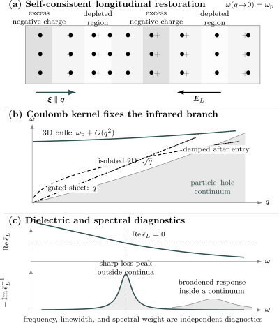
Three views of plasmon identification. A longitudinal density modulation creates a self-consistent electric restoring field. The Coulomb kernel sets the infrared dispersion: a three-dimensional bulk mode approaches $\omega_{\mathrm p}$, an isolated two-dimensional mode scales as $\sqrt q$, and a gate-screened mode is acoustic. A sharp mode appears as a complex dielectric zero and, under suitable probe conditions, as a peak in $-\operatorname{Im}\epsilon_L^{-1}$; entry into the particle–hole continuum broadens it.

Three-Dimensional Electron Gas

Long-wavelength dispersion

For a homogeneous, degenerate, three-dimensional electron gas with a parabolic band, collisionless RPA gives the small-$q$ expansion

$$\omega_{\mathrm{pl}}^2(q) = \omega_{\mathrm p}^2 + \frac35v_F^2q^2 + O(q^4).$$

Equivalently,

$$\omega_{\mathrm{pl}}(q) = \omega_{\mathrm p} \left[ 1+ \frac3{10} \frac{v_F^2q^2}{\omega_{\mathrm p}^2} +O(q^4) \right].$$

The coefficient $3v_F^2/5$ is a collisionless Fermi-surface result. It is not the ordinary hydrodynamic sound speed obtained from an isothermal or adiabatic equation of state. The limits

$$\omega\tau_{\mathrm{coll}}\gg1 \qquad\text{and}\qquad \omega\tau_{\mathrm{coll}}\ll1$$

probe different pressure closures and need not give the same $q^2$ correction.

The Random Phase Approximation page derives this expansion from the Lindhard polarization. The nonzero intercept follows more generally from charge conservation, long-range Coulomb forces, and the longitudinal oscillator-strength sum rule.

Where the branch meets microscopic excitations

For a parabolic band at zero temperature, the upper boundary of the one-pair intraband continuum is

$$\omega_+(q) = v_Fq + \frac{\hbar q^2}{2m}.$$

A rough onset estimate follows by comparing

$$\omega_{\mathrm p} \sim v_Fq.$$

This suggests the scale

$$q_{\mathrm L} \sim \frac{\omega_{\mathrm p}}{v_F},$$

but it is not an exact threshold. The plasmon itself disperses, the continuum has curved boundaries, and correlations can broaden both structures. An actual threshold must be found from the complex dielectric function at the chosen density and temperature.

What is protected and what is model dependent

For a translationally invariant continuum of identical particles with a parabolic kinetic energy, the long-wavelength oscillator strength contains the bare inertial mass. Interactions redistribute spectral weight but do not freely renormalize the exact longitudinal $q\to0$ plasma scale.

That statement changes in a crystal. A lattice breaks Galilean invariance, and the low-energy charge stiffness is controlled by the optical or Drude weight rather than by replacing $m$ mechanically with a quasiparticle effective mass. Interband polarization also changes the background dielectric environment.

Thus one should distinguish

$$\begin{gathered} \text{continuum bare mass}, \\ \text{band curvature}, \\ \text{optical mass or Drude weight}, \\ \text{quasiparticle effective mass}. \end{gathered}$$

They coincide only in restricted models.

Local-field corrections, vertex corrections, and short-range correlations can change the finite-$q$ dispersion, linewidth, and pole weight. The existence of a sharp branch at a given $q$ is therefore less universal than the leading bulk plasma scale.

Two-Dimensional and Dirac Systems

Isolated parabolic sheet

Place a two-dimensional carrier sheet between two simple dielectrics and neglect retardation. At long wavelength, write their effective relative permittivity as

$$\epsilon_{\mathrm{eff}} = \frac{\epsilon_1+\epsilon_2}{2}.$$

The sheet Coulomb kernel is

$$v_q^{2\mathrm D} = \frac{Q^2} {2\epsilon_0\epsilon_{\mathrm{eff}}q}.$$

Combining it with the inertial density response gives

$$\omega_{\mathrm{pl}}^2(q) = \frac{n_{2\mathrm D}Q^2q} {2m\epsilon_0\epsilon_{\mathrm{eff}}}.$$

Hence

$$\omega_{\mathrm{pl}}(q) \propto \sqrt q.$$

There is no contradiction with the finite three-dimensional bulk gap. The electronic motion is two-dimensional, but its electric field spreads through three-dimensional space, changing the Coulomb kernel from $q^{-2}$ to $q^{-1}$.

Drude-weight formulation

The parabolic expression is not the best starting point for a nonparabolic band. Define the collisionless longitudinal sheet conductivity by

$$\sigma_L(\omega) \simeq \frac{i\mathcal D} {\pi(\omega+i0^+)}.$$

This equation fixes the convention for the sheet Drude weight $\mathcal D$. Continuity and electrostatics then give

$$\omega_{\mathrm{pl}}^2(q) = \frac{\mathcal Dq} {2\pi\epsilon_0\epsilon_{\mathrm{eff}}}.$$

For a parabolic sheet,

$$\mathcal D = \frac{\pi n_{2\mathrm D}Q^2}{m},$$

which recovers the preceding result.

This form is especially useful for Dirac and multiband systems. Band geometry, carrier density, temperature, interactions, and degeneracy enter through $\mathcal D$. The $\sqrt q$ law can survive even when no constant band mass exists.

Drude-weight conventions differ by factors of $\pi$ across the literature. A numerical formula is incomplete unless the conductivity convention is stated with it.

Thickness and dielectric environment

A real quantum well or layered material is not an infinitely thin sheet. Its interaction can be written schematically as

$$v_q = \frac{Q^2} {2\epsilon_0\epsilon_{\mathrm{eff}}q} F(q),$$

where $F(q)\to1$ as the wavelength becomes much longer than the layer thickness. At larger $q$, the transverse wave function and nearby interfaces matter.

The simple average $(\epsilon_1+\epsilon_2)/2$ also assumes local, frequency-independent half-spaces and a single interface geometry. Anisotropic substrates, polar phonons, metallic gates, and layered dielectrics produce a $q$- and $\omega$-dependent environmental kernel.

Density scaling

For a parabolic two-dimensional gas,

$$\omega_{\mathrm{pl}} \propto n_{2\mathrm D}^{1/2}q^{1/2}.$$

For a doped two-dimensional Dirac cone, the Drude weight scales with Fermi energy. Since

$$E_F\propto\sqrt{n_{2\mathrm D}},$$

the long-wavelength plasmon instead scales as

$$\omega_{\mathrm{pl}} \propto n_{2\mathrm D}^{1/4}q^{1/2}$$

within the ideal low-temperature Dirac regime. The different density exponent is a direct probe of band kinematics, not a change in the spatial Coulomb law.

Surface and Electromagnetic Modes

Nonretarded planar surface mode

Consider a flat interface between a local metal with dielectric function $\epsilon_m(\omega)$ and a dielectric with $\epsilon_d(\omega)$. In the electrostatic limit, a bound interface solution obeys

$$\epsilon_m(\omega) + \epsilon_d(\omega) =0.$$

Introduce an unscreened oscillator-strength frequency

$$\omega_{p0}^2 = \frac{n_0Q^2}{m\epsilon_0}$$

and the lossless local model

$$\epsilon_m(\omega) = \epsilon_\infty - \frac{\omega_{p0}^2}{\omega^2}.$$

For a frequency-independent exterior dielectric, the surface-mode frequency is

$$\omega_s = \frac{\omega_{p0}} {\sqrt{\epsilon_\infty+\epsilon_d}}.$$

If $\epsilon_\infty=\epsilon_d=1$, this becomes

$$\omega_s = \frac{\omega_{p0}}{\sqrt2}.$$

The bulk longitudinal zero of the same local metal is instead

$$\omega_{\mathrm{bulk}} = \frac{\omega_{p0}}{\sqrt{\epsilon_\infty}}.$$

The familiar factor $1/\sqrt2$ is therefore not a universal surface-plasmon rule. It assumes vacuum on both sides of the oscillator-strength bookkeeping and neglects damping, spatial dispersion, and interband structure.

Retarded surface plasmon polariton

Retaining Maxwell retardation gives the planar transverse-magnetic surface-polariton dispersion

$$q(\omega) = \frac{\omega}{c} \sqrt{ \frac{\epsilon_m(\omega)\epsilon_d(\omega)} {\epsilon_m(\omega)+\epsilon_d(\omega)} }.$$

For a lossless interface, confinement requires the fields to decay away from the interface. In the usual positive-dielectric case, this entails approximately

$$\operatorname{Re}\epsilon_m < -\epsilon_d.$$

At small $q$, the branch approaches the light line and is strongly electromagnetic. At large $q$, the local model approaches the nonretarded condition $\epsilon_m+\epsilon_d=0$.

The branch is therefore a surface plasmon polariton, not a purely electrostatic density oscillator. Its propagation length, mode confinement, and radiative coupling require the full boundary-value problem.

Localized surface resonances

A finite particle supports localized charge oscillations whose resonance condition depends on shape. For one quasistatic polarization axis of an ellipsoid,

$$\epsilon_d + L \left( \epsilon_m-\epsilon_d \right) =0,$$

where $L$ is the depolarization factor along that axis. For a sphere, $L=1/3$, giving

$$\epsilon_m+2\epsilon_d=0.$$

Shape, size, retardation, radiation, nonlocality, and the surrounding dielectric all shift and broaden localized resonances. They should not be identified by inserting a bulk plasma frequency into a universal formula.

Multicomponent and Hybrid Modes

Dielectric matrices

With several layers, bands, valleys, or carrier fluids, the response is matrix valued. A collective mode satisfies

$$\sum_b \epsilon_{ab}(\mathbf q,\omega) \phi_b =0,$$

and therefore

$$\det\boldsymbol\epsilon(\mathbf q,\omega) =0.$$

The eigenvector $\boldsymbol\phi$ determines how the component densities move relative to one another. A determinant zero alone does not say which experimental vertex couples strongly to that eigenvector.

Charged and nearly neutral combinations

For several mobile fluids, a high-frequency eigenmode often carries a substantial net charge-density fluctuation. Its long-wavelength scale is schematically

$$\omega_+^2 \simeq \sum_a \frac{n_aQ_a^2} {m_a\epsilon_0\epsilon_{\mathrm b}}.$$

Another eigenvector can move the components so their charge fluctuations nearly cancel. Such an out-of-phase branch can remain acoustic:

$$\omega_-(q) \simeq c_-q.$$

Whether it is sharp depends on the particle–hole continua of every component. A mathematically valid acoustic root can be so strongly Landau damped that it is not a useful quasiparticle.

Examples include bilayer acoustic plasmons, electron–hole fluids, and multiband metals. The labels in phase and out of phase must be interpreted together with the signs of the component charges.

Plasmon–phonon hybridization

In a polar material, a charge oscillation can couple to a longitudinal optical phonon. A minimal lossless model for the squared frequencies is

$$\begin{pmatrix} \omega_{\mathrm{pl}}^2(q) & \Lambda(q) \\ \Lambda(q) & \omega_{\mathrm{ph}}^2(q) \end{pmatrix},$$

where $\Lambda$ has units of frequency squared. The hybrid eigenfrequencies are

$$\begin{aligned} \omega_\pm^2 ={}& \frac12 \left( \omega_{\mathrm{pl}}^2 + \omega_{\mathrm{ph}}^2 \right) \\ &\pm \frac12 \sqrt{ \left( \omega_{\mathrm{pl}}^2 - \omega_{\mathrm{ph}}^2 \right)^2 +4\Lambda^2 }. \end{aligned}$$

Near the uncoupled crossing, the branches repel and exchange charge and lattice character. Consequently, their frequencies, linewidths, and probe intensities evolve together.

With damping, the effective matrix is non-Hermitian. The real-frequency peak separation can disappear before the complex poles coalesce, and a two-Lorentzian fit need not recover the true eigenmodes.

Charged superfluids

A neutral superfluid has a gapless phase mode. Long-range Coulomb forces attach a self-consistent electric field to charge-phase motion and raise the longitudinal mode to a plasma scale. This is the condensed-matter Anderson–Higgs mechanism.

The Goldstone Modes in Many-Body Systems page owns the symmetry argument. The important point here is that superconductivity does not create the entire plasma frequency from nothing; it reorganizes the charged phase response and spectral weight subject to gauge invariance and electrodynamics.

Quantization and Effective Description

Projecting the density onto a sharp branch

Let the per-particle dynamic structure factor use the convention

$$S_n(\mathbf q,\omega) = \frac1N \sum_m \left| \langle m|\rho_{\mathbf q}|0\rangle \right|^2 \delta(\omega-\omega_{m0}),$$

where

$$\rho_{\mathbf q} = \sum_{j=1}^N e^{-i\mathbf q\cdot\mathbf r_j}.$$

If one mode contributes weight $Z_n(q)$, then

$$\left| \langle\mathrm{pl},\mathbf q| \rho_{\mathbf q}|0\rangle \right|^2 = NZ_n(q).$$

Within the one-mode subspace, one may write

$$\rho_{\mathbf q} \simeq \sqrt{NZ_n(q)} \left( b_{\mathbf q} + b_{-\mathbf q}^\dagger \right),$$

up to phase and normalization conventions. This relation makes clear why a long-wavelength bulk plasmon can have a finite energy but density matrix element vanishing as $q$.

Beyond the harmonic mode

The harmonic Hamiltonian does not determine the lifetime. Anharmonic terms have the schematic form

$$\begin{aligned} H_{\mathrm{int}} ={}& \sum_{123} g^{(3)}_{123} b_1^\dagger b_2b_3 \\ &+ \sum_{1234} g^{(4)}_{1234} b_1^\dagger b_2^\dagger b_3b_4 +\cdots. \end{aligned}$$

They allow decay, scattering, frequency shifts, and nonlinear response when conservation laws and phase space permit. Coupling to particle–hole and interband continua adds nonlocal-in-time self-energies rather than a single constant damping rate.

At high occupation, the same mode can often be described as a classical coherent charge oscillation. A plasmon number state, a coherent plasmon field, and a driven dissipative steady state are different quantum states even when they share the same linear resonance frequency.

Experimental Diagnostics

Electron energy-loss spectroscopy

A fast charged particle carries an electric field with longitudinal components and can transfer both energy and momentum to the sample. In a simple homogeneous bulk geometry, the loss probability contains the energy-loss function

$$\mathcal L(\mathbf q,\omega) = -\operatorname{Im} \frac1{\epsilon_L^{\mathrm{phys}}(\mathbf q,\omega)}.$$

A sharp maximum in $\mathcal L$ is a classic plasmon signature. Yet the measured spectrum also contains kinematic factors, multiple scattering, surface losses, finite-thickness interference, instrumental broadening, and the momentum acceptance of the spectrometer.

Transmission electron energy-loss spectroscopy can sample bulk and surface excitations. Reflection geometries emphasize boundary response. A feature observed in both is not automatically the same eigenmode; the electromagnetic boundary-value problem decides the mixture.

Inelastic x-ray scattering

Nonresonant inelastic x-ray scattering couples primarily to electron density and measures a cross section proportional to a dynamic structure factor after known kinematic factors are removed:

$$\frac{d^2\sigma} {d\Omega\,d\omega} \propto S_n(\mathbf q,\omega).$$

This gives direct access to finite momentum and can follow a plasmon into a particle–hole continuum. Core-electron backgrounds, form factors, resolution, and the distinction between valence and total density must still be handled.

The loss function and the structure factor are related through response theory, but they are not identical functions. Their peak positions are often close for a weakly damped isolated pole and can differ substantially in a structured, lossy, or multicomponent medium.

Optical spectroscopy

Far-field light carries very small crystal momentum on electronic scales:

$$q_{\mathrm{photon}} \sim \frac{\omega}{c}.$$

Reflectivity, ellipsometry, and transmission determine transverse optical response and can reveal a plasma edge, screened plasma frequency, or plasmon–phonon hybrid. A homogeneous bulk longitudinal plasmon is not directly excited by a perfectly transverse plane wave in an infinite medium.

Surfaces, finite incidence angle, disorder, gratings, and patterning can supply longitudinal fields or additional momentum. Interpreting an optical minimum or reflectivity edge as a longitudinal dielectric zero therefore requires a Maxwell model of the actual sample.

Momentum-enhancing probes

Near-field microscopy, patterned couplers, electron beams, and nanostructures can access momenta far beyond the free-space light line. Raman scattering can reveal symmetry-selected low-momentum electronic collective modes, while resonant x-ray techniques add orbital and element selectivity.

Every probe measures a vertex-dressed correlation function. A weak peak can mean

• little mode spectral weight;
• a small coupling vertex;
• destructive matrix-element interference;
• strong damping;
• poor momentum matching;
• polarization mismatch;
• instrumental resolution broader than the intrinsic line.

Absence of a peak in one channel is not proof that no collective pole exists.

Minimal identification criteria

A persuasive plasmon assignment should establish several of the following:

1. a dispersion consistent with the dimensional Coulomb kernel;
2. a dielectric zero or screened-response pole at complex frequency;
3. a loss or density peak with compatible energy and linewidth;
4. charge-density character in the mode eigenvector;
5. spectral weight consistent with an appropriate sum rule;
6. evolution relative to particle–hole and interband continua;
7. dependence on carrier density, dielectric environment, or gate distance;
8. agreement across probes after their different vertices are modeled.

One peak at one momentum is rarely enough to determine all of these.

Approximation Ladder

Hydrodynamics and local electrodynamics

Hydrodynamics gives the leading restoring mechanism and dimensional scaling with very little microscopic input. It is strongest when the wavelength is long, the relevant conservation laws are known, and a controlled closure for pressure and dissipation exists.

It cannot by itself determine the particle–hole continuum, quantum spectral weight distribution, interband matrix elements, or a collisionless Landau-damping rate.

Kinetic theory and RPA

Kinetic theory resolves the distribution function in phase space. RPA resolves the noninteracting quantum polarization and sums the self-consistent Coulomb field. For a weakly or moderately correlated electron gas, RPA captures

• the bulk plasma gap;
• the leading long-wavelength dispersion;
• dimensional plasmon scaling;
• collisionless particle–hole continua;
• one-pair Landau damping;
• screening and dielectric zeros.

Its controlled regimes and diagrammatic meaning are developed on the Random Phase Approximation page.

Conserving approximations

Once self-energies dress propagators, vertices must generally be treated consistently. Charge conservation imposes Ward identities connecting density and current response. An arbitrary dressed bubble can violate continuity, the compressibility relation, or the $f$-sum rule.

Baym–Kadanoff conserving constructions, kinetic equations with consistent collision integrals, and gauge-invariant vertex schemes are designed to preserve these constraints. Passing a sum rule is necessary but not sufficient for complete accuracy.

Local-field and exchange-correlation corrections

Short-range exchange and correlation can be represented through local-field factors or exchange-correlation kernels:

$$\bar\epsilon_L = 1- v_q \left[ 1-G(q,\omega) \right] \Pi_0(q,\omega),$$

in one common schematic convention. Different definitions move factors between $G$, the irreducible polarization, and the kernel.

Time-dependent density-functional theory uses an exchange-correlation kernel $f_{\mathrm{xc}}$ rather than a bare RPA denominator. Static local-field models can improve some dispersions yet miss memory and multipair damping.

First-principles dielectric matrices

In a crystal, microscopic fields mix reciprocal lattice vectors:

$$\epsilon_{\mathbf G\mathbf G'} (\mathbf q,\omega).$$

Macroscopic response is not generally the $\mathbf G=\mathbf G'=0$ matrix element of $\boldsymbol\epsilon$. Instead, a common longitudinal definition is

$$\epsilon_M(\mathbf q,\omega) = \frac1{ \epsilon^{-1}_{00}(\mathbf q,\omega) }.$$

Off-diagonal reciprocal-lattice components encode crystal local-field effects. Band structure, interband transitions, spin–orbit coupling, dimensional truncation of Coulomb interactions, and matrix elements all matter.

Density-functional perturbation theory, time-dependent density-functional theory, $GW$-based response, and Bethe–Salpeter methods form a hierarchy rather than interchangeable black boxes. Numerical convergence in empty bands, momentum mesh, frequency grid, broadening, and Coulomb treatment must accompany a claimed plasmon energy.

Controlled Limits and Consistency Checks

Neutrality and the uniform component

An infinite Coulomb system requires a neutralizing background or an explicit finite-geometry electrostatic problem. The $\mathbf q=0$ Coulomb component is normally removed from the neutral periodic Hamiltonian.

The rule

$$\rho_{\mathbf q=0}=Q\hat N$$

then expresses a conserved total charge, not a finite-frequency oscillator. The bulk plasma frequency belongs to a sequence of neutral, nonuniform fluctuations whose wavelength tends to infinity.

Dimensional analysis

In three dimensions,

$$\frac{n_0Q^2} {m\epsilon_0}$$

has units of inverse time squared. In a two-dimensional sheet, one additional factor of $q$ is required:

$$\frac{n_{2\mathrm D}Q^2q} {m\epsilon_0}.$$

A proposed two-dimensional plasmon frequency independent of $q$ must therefore contain another inverse length, such as gate distance, layer spacing, or a three-dimensional carrier density.

Causality and passivity

With the $e^{-i\omega t}$ convention, a retarded dielectric response is analytic for

$$\operatorname{Im}\omega>0.$$

For a passive homogeneous medium at positive real frequency, the correctly normalized loss function should be nonnegative:

$$-\operatorname{Im} \epsilon_L^{-1}(\mathbf q,\omega) \ge0.$$

Real and imaginary parts are related by Kramers–Kronig relations. A fitted real dielectric zero accompanied by the wrong sign of absorption, or by poles in the upper half-plane, is unphysical.

Sum-rule audit

Integrating the complete density spectrum must recover the appropriate first moment. A model that includes only the plasmon pole should state the fraction of the sum rule it exhausts:

$$\eta_{\mathrm{pl}}(q) := \frac{ \omega_{\mathrm{pl}}(q)Z_n(q) }{ \hbar q^2/(2m) }.$$

For exact single-mode saturation,

$$\eta_{\mathrm{pl}}=1.$$

At finite $q$, omitted continua and interband excitations generally make $\eta_{\mathrm{pl}}<1$ for the isolated pole.

Static and dynamic limits

The two limits

$$\lim_{q\to0}\lim_{\omega\to0} \qquad\text{and}\qquad \lim_{\omega\to0}\lim_{q\to0}$$

need not agree. The first can probe equilibrium screening or compressibility, whereas the second can probe a spatially uniform dynamical field constrained by conservation laws.

Replacing a dynamic dielectric function by its static value inside a plasmon equation can remove the mode one is trying to calculate.

Electrostatic and retarded limits

The electrostatic approximation requires the mode momentum to be large compared with the light-line momentum in its environment:

$$q \gg \frac{\sqrt{\epsilon}\,\omega}{c}.$$

Near the light line, longitudinal and transverse fields hybridize and a full Maxwell treatment is required. Conversely, applying a purely photonic polariton formula deep in the nonretarded regime can obscure the many-body density response.

Continuum and linewidth check

For each candidate mode, plot it together with all allowed intraband, interband, phonon, and multipair continua. Then ask whether

$$\gamma_{\mathrm{pl}} \ll \Omega_{\mathrm{pl}}.$$

A real root outside every one-pair continuum can still decay through disorder, multipair production, phonons, or radiation. A mode inside a continuum can remain visible if coupling and phase space are weak, but it is not protected merely because a real-part equation has a solution.

Worked Examples

Free-electron bulk estimate

Take

$$n_0 = 1.81\times10^{29}\ {\mathrm m}^{-3}, \qquad \epsilon_{\mathrm b}=1,$$

and use the electron mass. Then

$$\begin{aligned} \omega_{\mathrm p} &= \sqrt{ \frac{n_0e^2}{m_e\epsilon_0} }, \\ &\simeq 2.40\times10^{16}\ {\mathrm s}^{-1}. \end{aligned}$$

The corresponding energy is

$$\hbar\omega_{\mathrm p} \simeq 15.8\ {\mathrm{eV}}.$$

This is the familiar scale for a simple high-density metal. It is a free-electron estimate, not a substitute for an optical dielectric calculation: interband polarization, band structure, and damping shift the observed loss maximum.

Density change in bulk and in a Dirac sheet

For a parabolic three-dimensional plasma at fixed mass and background dielectric,

$$\omega_{\mathrm p}\propto n_0^{1/2}.$$

Increasing density by a factor of four doubles the plasma frequency.

For an ideal doped two-dimensional Dirac system at fixed $q$ and dielectric environment,

$$\omega_{\mathrm{pl}}\propto n_{2\mathrm D}^{1/4}.$$

The same fourfold density increase gives only

$$4^{1/4}=\sqrt2$$

times the frequency. Measuring the density exponent can help distinguish band kinematics, provided the dielectric environment and scattering do not change simultaneously.

Gate crossover

For a sheet a distance $d$ from an ideal metallic gate,

$$v_q^{\mathrm{gate}} = \frac{Q^2} {2\epsilon_0\epsilon_{\mathrm{eff}}q} \left( 1-e^{-2qd} \right).$$

If $qd\ll1$,

$$1-e^{-2qd} \simeq 2qd,$$

so

$$v_q^{\mathrm{gate}} \simeq \frac{Q^2d} {\epsilon_0\epsilon_{\mathrm{eff}}}.$$

The long-wavelength mode is therefore

$$\omega_{\mathrm{gate}}(q) \simeq c_{\mathrm{gate}}q,$$

with

$$c_{\mathrm{gate}} = \sqrt{ \frac{n_{2\mathrm D}Q^2d} {m\epsilon_0\epsilon_{\mathrm{eff}}} }.$$

For $qd\gg1$, the exponential is negligible and the isolated $\sqrt q$ behavior returns. The crossover momentum is of order $d^{-1}$.

Surface frequency with background screening

Suppose

$$\epsilon_\infty=4, \qquad \epsilon_d=2.25.$$

The bulk longitudinal frequency of the local Drude metal is

$$\omega_{\mathrm{bulk}} = \frac{\omega_{p0}}2,$$

whereas the nonretarded surface frequency is

$$\omega_s = \frac{\omega_{p0}}{\sqrt{6.25}} = \frac{\omega_{p0}}{2.5}.$$

Thus

$$\frac{\omega_s}{\omega_{\mathrm{bulk}}} = 0.8,$$

not $1/\sqrt2$. The dielectric environment changes the ratio.

Long-wavelength pole weight

If a three-dimensional plasmon exhausts the density first moment,

$$Z_n(q) = \frac{\hbar q^2} {2m\omega_{\mathrm p}} +O(q^4).$$

The excitation energy stays finite, but its density weight vanishes as $q^2$. At exactly $q=0$, the density operator is total particle number and cannot create the mode.

This is a useful example of why the existence of a finite-frequency limiting branch does not imply a finite matrix element for a uniform density perturbation.

Common Mistakes

Treating every loss peak as a plasmon

Interband transitions, excitons, phonons, multiple scattering, and instrumental artifacts can all produce peaks. Establish charge collectivity, dispersion, and dielectric structure rather than assigning by energy alone.

Solving only the real-part equation

The condition

$$\operatorname{Re}\epsilon_L(q,\omega)=0$$

does not determine a mode when $\operatorname{Im}\epsilon_L$ is large. Locate the complex pole or zero and inspect the full spectral function.

Confusing the bulk, screened, and surface frequencies

The quantities

$$\omega_{p0}, \qquad \frac{\omega_{p0}}{\sqrt{\epsilon_\infty}}, \qquad \frac{\omega_{p0}} {\sqrt{\epsilon_\infty+\epsilon_d}}$$

refer to different electrodynamic problems.

Replacing the mass without checking a sum rule

In a continuum Galilean-invariant liquid, the long-wavelength oscillator strength involves the bare inertial mass. In a lattice, the Drude weight is the safer object. A single-particle quasiparticle mass is not automatically the optical mass.

Ignoring the dielectric environment

For a sheet, substrate, encapsulation, gates, and nearby polar modes can alter both frequency and damping. Quoting only carrier density and an isolated-layer formula is incomplete.

Calling every linear mode neutral sound

A gate-screened plasmon can be acoustic in dispersion while still carrying charge and electric-field energy. Acoustic describes $\omega\propto q$; it does not determine the eigenvector.

Equating loss function and structure factor

Both can reveal the same weakly damped mode, but their residues, backgrounds, and even apparent maxima can differ.

Forgetting the exact uniform mode

The operator $\rho_{\mathbf0}$ is conserved in a closed number-conserving system. The bulk plasma gap is a $q\to0$ result.

Ignoring damping outside the one-pair continuum

Disorder, phonons, multipair states, interband absorption, and radiative loss remain available.

Using one broadening parameter as microscopic proof

A phenomenological $\Gamma$ can fit a line without identifying whether the underlying process is elastic, inelastic, homogeneous, or instrumental.

Applying local electrodynamics at arbitrary momentum

Spatial dispersion matters when the wavelength approaches microscopic scales. Conversely, retardation matters near the light line.

Reading an avoided crossing as two uncoupled modes

Hybrid branches exchange spectral weight and character. Tracking only peak order can silently swap mode identities.

Decision Checklist

Before calling a feature a plasmon, specify:

• the dimensionality of carrier motion and electric fields;
• the Coulomb kernel and electromagnetic unit system;
• carrier densities, charges, and inertial or Drude weights;
• background, substrate, gate, and boundary dielectric response;
• whether the calculation is electrostatic or retarded;
• the response function whose zero, pole, or peak is being tracked;
• the particle–hole and interband continua;
• the complex frequency and linewidth convention;
• the fraction of the relevant sum rule carried by the feature;
• the probe vertex and experimental momentum resolution;
• the approximation used for self-energy and vertex corrections;
• which frequency is meant by bulk, screened, surface, or polaritonic.

This ledger prevents most factor, sign, and interpretation errors before detailed numerics begin.

Exercises

Exercise 1: Bulk plasma frequency from fluid equations

Consider a three-dimensional fluid of particles with equilibrium density $n_0$, charge $Q$, mass $m$, and background relative permittivity $\epsilon_{\mathrm b}$. Neglect pressure and damping.

Starting from continuity, force balance, and Gauss’s law, derive the longitudinal bulk plasma frequency. Explain why its sign is independent of whether the mobile carriers are positively or negatively charged.

Solution

The linearized equations are

$$\partial_t\delta n + n_0\nabla\cdot\mathbf u =0,$$ $$m\partial_t\mathbf u = Q\mathbf E,$$

and

$$\nabla\cdot\mathbf E = \frac{Q\delta n} {\epsilon_0\epsilon_{\mathrm b}}.$$

Differentiate continuity once:

$$\partial_t^2\delta n + n_0\nabla\cdot \partial_t\mathbf u =0.$$

Use force balance:

$$\partial_t^2\delta n + \frac{n_0Q}{m} \nabla\cdot\mathbf E =0.$$

Gauss’s law then gives

$$\partial_t^2\delta n + \frac{n_0Q^2} {m\epsilon_0\epsilon_{\mathrm b}} \delta n =0.$$

Thus

$$\omega_{\mathrm p}^2 = \frac{n_0Q^2} {m\epsilon_0\epsilon_{\mathrm b}}.$$

The density fluctuation creates charge density $Q\delta n$, and the resulting electric field exerts force $Q\mathbf E$. These two factors multiply to $Q^2$, so reversing the carrier charge reverses both the field source and the force direction, leaving the restoring frequency unchanged.

Exercise 2: Coulomb kernel and dimensional scaling

Assume a long-wavelength density mode obeys

$$\omega^2(q) \simeq \frac{n_d}{m} q^2v_q.$$

Find the infrared dispersion for each kernel:

$$\begin{aligned} v_q^{(a)}&=\frac{C_3}{q^2}, \\ v_q^{(b)}&=\frac{C_2}{q}, \\ v_q^{(c)}&=C_0, \\ v_q^{(d)}&=C_1\ln\frac1{qa}. \end{aligned}$$

Identify the usual physical setting for each result.

Solution

For kernel (a),

$$\omega^2 \simeq \frac{n_dC_3}{m},$$

so

$$\omega(q\to0) \to \text{constant}.$$

This is the three-dimensional bulk Coulomb plasma.

For kernel (b),

$$\omega^2 \simeq \frac{n_dC_2}{m}q,$$

and therefore

$$\omega\propto\sqrt q.$$

This is an isolated two-dimensional sheet whose electric field occupies three-dimensional space.

For kernel (c),

$$\omega^2 \simeq \frac{n_dC_0}{m}q^2,$$

so

$$\omega\propto q.$$

This describes a short-range interaction or a Coulomb interaction screened to a constant at small $q$, as for a nearby ideal gate.

For kernel (d),

$$\omega(q) \simeq q \sqrt{ \frac{n_dC_1}{m} \ln\frac1{qa} }.$$

This is the characteristic quasi-one-dimensional Coulomb result: it is nearly acoustic, with a logarithmically increasing phase velocity as $q\to0$. The transverse length $a$ regularizes the short-distance interaction.

Exercise 3: Exactly uniform density

Let

$$\rho_{\mathbf q} = \sum_{j=1}^N e^{-i\mathbf q\cdot\mathbf r_j}.$$

Show that a number-conserving closed system has no positive-frequency density spectral weight at exactly $\mathbf q=0$. Reconcile this result with a finite three-dimensional limit $\omega_{\mathrm{pl}}(q\to0)=\omega_{\mathrm p}$.

Solution

At zero momentum,

$$\rho_{\mathbf0} = \sum_{j=1}^N1 = \hat N.$$

Number conservation gives

$$[H,\hat N]=0.$$

Choose energy eigenstates that also diagonalize $\hat N$. Within a fixed-$N$ sector,

$$\langle m|\hat N|0\rangle = N\langle m|0\rangle =0$$

for every excited state $m\ne0$. Therefore

$$S_n(\mathbf0,\omega>0)=0.$$

For every nonzero but arbitrarily small $q$, $\rho_{\mathbf q}$ is not the conserved total number. It can excite a longitudinal charge oscillation at a frequency approaching $\omega_{\mathrm p}$. Its one-mode matrix element simultaneously vanishes:

$$Z_n(q) \simeq \frac{\hbar q^2} {2m\omega_{\mathrm p}}.$$

Thus the mode frequency has a finite $q\to0$ limit while the density spectral weight tends to zero. There is no discontinuity in the exact conserved operator at $q=0$.

Exercise 4: Gate-induced acoustic plasmon

A parabolic carrier sheet with density $n_{2\mathrm D}$ lies a distance $d$ from an ideal metallic gate. Its electrostatic kernel is

$$v_q = \frac{Q^2} {2\epsilon_0\epsilon_{\mathrm{eff}}q} \left( 1-e^{-2qd} \right).$$

Derive the long-wavelength mode velocity and identify the crossover scale to the isolated-sheet regime.

Solution

For $qd\ll1$,

$$1-e^{-2qd} = 2qd+O(q^2d^2).$$

Hence

$$v_q \simeq \frac{Q^2d} {\epsilon_0\epsilon_{\mathrm{eff}}}.$$

Use the inertial density formula

$$\omega^2 \simeq \frac{n_{2\mathrm D}}m q^2v_q.$$

This gives

$$\omega(q) \simeq q \sqrt{ \frac{n_{2\mathrm D}Q^2d} {m\epsilon_0\epsilon_{\mathrm{eff}}} }.$$

Therefore the acoustic velocity is

$$c_{\mathrm{gate}} = \sqrt{ \frac{n_{2\mathrm D}Q^2d} {m\epsilon_0\epsilon_{\mathrm{eff}}} }.$$

For $qd\gg1$, the exponential image term is negligible and

$$v_q \simeq \frac{Q^2} {2\epsilon_0\epsilon_{\mathrm{eff}}q},$$

which restores $\omega\propto\sqrt q$. The crossover is parametrically

$$q_{\mathrm{cross}} \sim d^{-1}.$$

Exercise 5: Complex Drude zero

For

$$\bar\epsilon_L(\omega) = 1- \frac{\omega_{\mathrm p}^2} {\omega(\omega+i\Gamma)},$$

find the positive-frequency complex zero. Determine the weak-damping decay rate, full width at half maximum under the narrow-line approximation, and quality factor.

Solution

The zero condition is

$$\omega^2+i\Gamma\omega -\omega_{\mathrm p}^2 =0.$$

The root with positive real part is

$$\omega_* = \sqrt{ \omega_{\mathrm p}^2 -\frac{\Gamma^2}{4} } -\frac{i\Gamma}{2}.$$

Writing

$$\omega_* = \Omega_{\mathrm{pl}} -i\gamma_{\mathrm{pl}},$$

one has

$$\gamma_{\mathrm{pl}} = \frac\Gamma2.$$

For a narrow Lorentzian in angular frequency,

$$\mathrm{FWHM}_\omega \simeq 2\gamma_{\mathrm{pl}} = \Gamma.$$

The quality factor in the convention used on this page is

$$\mathcal Q = \frac{\Omega_{\mathrm{pl}}} {2\gamma_{\mathrm{pl}}} = \frac{ \sqrt{\omega_{\mathrm p}^2-\Gamma^2/4} }{\Gamma}.$$

An oscillatory root requires

$$\Gamma<2\omega_{\mathrm p},$$

whereas a well-defined narrow plasmon requires the stronger condition

$$\Gamma\ll\omega_{\mathrm p}.$$

Exercise 6: Two-dimensional pole weight

An isolated parabolic two-dimensional plasmon has

$$\omega_{\mathrm{pl}}(q) = A\sqrt q.$$

Assume it exhausts the per-particle density $f$-sum rule at sufficiently small $q$. Determine its pole weight $Z_n(q)$ and the scaling of its density matrix element.

Solution

Single-mode saturation gives

$$\omega_{\mathrm{pl}}(q)Z_n(q) = \frac{\hbar q^2}{2m}.$$

Therefore

$$Z_n(q) = \frac{\hbar} {2mA} q^{3/2}.$$

With the per-particle structure-factor convention,

$$\left| \langle\mathrm{pl},\mathbf q| \rho_{\mathbf q}|0\rangle \right|^2 = NZ_n(q).$$

Its magnitude scales as

$$\left| \langle\mathrm{pl},\mathbf q| \rho_{\mathbf q}|0\rangle \right| \propto \sqrt N\,q^{3/4}.$$

The plasmon softens as $\sqrt q$, but the density matrix element still vanishes. Energy and spectral weight have different infrared powers.

Exercise 7: Planar surface condition

Let a planar interface at $z=0$ separate a metal in $z<0$ from a dielectric in $z>0$. In the nonretarded, source-free regions, take potentials

$$\phi_m = A e^{qz}e^{i\mathbf q\cdot\mathbf r_\parallel}$$

and

$$\phi_d = B e^{-qz}e^{i\mathbf q\cdot\mathbf r_\parallel}.$$

Use the boundary conditions to derive the surface-mode condition. Then obtain the lossless Drude result for constant $\epsilon_d$.

Solution

Continuity of the potential at $z=0$ gives

$$A=B.$$

The normal electric fields are

$$E_{z,m} = -\partial_z\phi_m = -qA$$

and

$$E_{z,d} = -\partial_z\phi_d = +qB.$$

With no externally imposed free surface charge, the normal displacement is continuous:

$$\epsilon_mE_{z,m} = \epsilon_dE_{z,d}.$$

Using $A=B$ gives

$$-\epsilon_mqA = \epsilon_dqA.$$

A nonzero field therefore requires

$$\epsilon_m(\omega) + \epsilon_d(\omega) =0.$$

For

$$\epsilon_m(\omega) = \epsilon_\infty - \frac{\omega_{p0}^2}{\omega^2}$$

and constant $\epsilon_d$,

$$\epsilon_\infty+\epsilon_d - \frac{\omega_{p0}^2}{\omega^2} =0.$$

Thus

$$\omega_s = \frac{\omega_{p0}} {\sqrt{\epsilon_\infty+\epsilon_d}}.$$

Exercise 8: Estimate of continuum entry in a sheet

For a parabolic two-dimensional carrier gas, write

$$\omega_{\mathrm{pl}}^2(q) = Aq, \qquad A = \frac{n_{2\mathrm D}Q^2} {2m\epsilon_0\epsilon_{\mathrm{eff}}}.$$

At small $q$, approximate the upper intraband particle–hole scale by $v_Fq$. Estimate where the plasmon reaches this scale and explain why the mode begins above the continuum as $q\to0$.

Solution

Equate the two estimates:

$$\sqrt{Aq_{\mathrm L}} \sim v_Fq_{\mathrm L}.$$

For nonzero $q_{\mathrm L}$,

$$q_{\mathrm L} \sim \frac{A}{v_F^2}.$$

Substituting $A$ gives

$$q_{\mathrm L} \sim \frac{n_{2\mathrm D}Q^2} {2m\epsilon_0\epsilon_{\mathrm{eff}}v_F^2}.$$

The plasmon phase velocity is

$$\frac{\omega_{\mathrm{pl}}(q)}q = \sqrt{\frac Aq}.$$

It diverges as $q^{-1/2}$, while the characteristic particle–hole velocity remains $v_F$. Hence the ideal long-wavelength plasmon lies above the intraband continuum.

This is only a scaling estimate. The recoil term $\hbar q^2/(2m)$, the full polarization, finite temperature, interband transitions, disorder, and interaction corrections shift or smear the actual entry.

Summary

• A plasmon is the quantum of a collective charge-density oscillation supported by a self-consistent electric field.
• In a neutral three-dimensional parabolic continuum, long-range Coulomb forces give $\omega_{\mathrm{pl}}(q\to0)=\omega_{\mathrm p}$ with $\omega_{\mathrm p}^2=n_0Q^2/(m\epsilon_0\epsilon_{\mathrm b})$.
• Exactly $q=0$, density is the conserved total number; the finite plasma gap is a limit of nonuniform modes whose density weight vanishes.
• The infrared law follows from $q^2v_q$: bulk three-dimensional modes are gapped, isolated two-dimensional modes scale as $\sqrt q$, gate-screened sheets can be acoustic, and quasi-one-dimensional modes carry logarithmic corrections.
• In a crystal or nonparabolic band, the optical Drude weight is generally more fundamental than inserting a quasiparticle mass into a continuum formula.
• A collective mode is identified by a complex dielectric zero or screened-response pole; a real-axis zero alone is insufficient when absorption is large.
• Density structure factor, loss function, conductivity, reflectivity, and probe cross sections are related but not interchangeable observables.
• Plasmons lose coherence through particle–hole continua, interband transitions, phonons, disorder, multipair states, collisions, and radiation.
• Surface plasmons, surface plasmon polaritons, and localized surface resonances obey different boundary conditions.
• Multicomponent charge fluids and phonons produce hybrid eigenmodes that exchange frequency, linewidth, and spectral weight.
• Causality, passivity, continuity, dielectric units, and the $f$-sum rule provide nonnegotiable consistency checks.
• RPA gives the canonical microscopic weak-correlation derivation; material-specific plasmonics requires dielectric matrices, band structure, electromagnetic boundaries, and probe modeling.

References

1. L. Tonks and I. Langmuir, “Oscillations in ionized gases,” Physical Review 33, 195–210 (1929), doi:10.1103/PhysRev.33.195. Early plasma-oscillation analysis and the collective frequency scale.
2. D. Bohm and D. Pines, “A collective description of electron interactions. I. Magnetic interactions,” Physical Review 82, 625–634 (1951), doi:10.1103/PhysRev.82.625. First paper in the collective-coordinate program for the electron gas.
3. D. Pines and D. Bohm, “A collective description of electron interactions: II. Collective versus individual particle aspects of the interactions,” Physical Review 85, 338–353 (1952), doi:10.1103/PhysRev.85.338. Separation of collective plasma motion from individual-particle excitations.
4. D. Bohm and D. Pines, “A collective description of electron interactions: III. Coulomb interactions in a degenerate electron gas,” Physical Review 92, 609–625 (1953), doi:10.1103/PhysRev.92.609. Canonical many-electron treatment of plasma modes and residual interactions.
5. J. Lindhard, “On the properties of a gas of charged particles,” Kongelige Danske Videnskabernes Selskab, Matematisk-fysiske Meddelelser 28(8), 1–57 (1954), OSTI 4405425. Exact noninteracting polarization of the degenerate electron gas.
6. R. A. Ferrell, “Characteristic energy loss of electrons passing through metal foils. II. Dispersion relation and short wavelength cutoff for plasma oscillations,” Physical Review 107, 450–462 (1957), doi:10.1103/PhysRev.107.450. Bulk-plasmon dispersion and termination in electron-loss spectra.
7. R. H. Ritchie, “Plasma losses by fast electrons in thin films,” Physical Review 106, 874–881 (1957), doi:10.1103/PhysRev.106.874. Surface-loss modes in finite metallic films.
8. P. W. Anderson, “Plasmons, gauge invariance, and mass,” Physical Review 130, 439–442 (1963), doi:10.1103/PhysRev.130.439. Charged phase modes and the many-body origin of gauge-field mass.
9. F. Stern, “Polarizability of a two-dimensional electron gas,” Physical Review Letters 18, 546–548 (1967), doi:10.1103/PhysRevLett.18.546. Two-dimensional polarization and the $\sqrt q$ plasmon.
10. A. L. Fetter, “Electrodynamics of a layered electron gas. I. Single layer,” Annals of Physics 81, 367–393 (1973), doi:10.1016/0003-4916(73)90161-9. Self-consistent electrodynamics of a conducting sheet.
11. P. E. Batson and J. Silcox, “Experimental energy-loss function, $\operatorname{Im}[-1/\epsilon(q,\omega)]$, for aluminum,” Physical Review B 27, 5224–5239 (1983), doi:10.1103/PhysRevB.27.5224. Momentum-resolved measurement of bulk-plasmon dispersion and loss.
12. E. H. Hwang and S. Das Sarma, “Dielectric function, screening, and plasmons in two-dimensional graphene,” Physical Review B 75, 205418 (2007), doi:10.1103/PhysRevB.75.205418. Dirac-band polarization, screening, and graphene plasmons.
13. J. M. Pitarke, V. M. Silkin, E. V. Chulkov, and P. M. Echenique, “Theory of surface plasmons and surface-plasmon polaritons,” Reports on Progress in Physics 70, 1–87 (2007), doi:10.1088/0034-4885/70/1/R01. Comprehensive review of bulk, surface, and retarded interface modes.
14. F. J. García de Abajo, “Optical excitations in electron microscopy,” Reviews of Modern Physics 82, 209–275 (2010), doi:10.1103/RevModPhys.82.209. Electron-beam coupling to plasmons, polaritons, and nanostructure modes.
15. G. F. Giuliani and G. Vignale, Quantum Theory of the Electron Liquid (Cambridge University Press, 2005), doi:10.1017/CBO9780511619915. Response functions, sum rules, electron-liquid plasmons, and correlation corrections.
16. G. D. Mahan, Many-Particle Physics, 3rd ed. (Springer, 2000), doi:10.1007/978-1-4757-5714-9. Dielectric response, electron energy loss, optical conductivity, and coupled modes.
17. A. L. Fetter and J. D. Walecka, Quantum Theory of Many-Particle Systems (McGraw–Hill, 1971). Linear response, the electron gas, RPA, collective modes, and conserving constraints.

Cross-Links

• Collective Modes
• Quasiparticles Overview
• Particle–Hole Excitations
• Random Phase Approximation
• Density Operators and Current Operators
• Susceptibilities
• Retarded and Advanced Response
• Structure Factors
• Sum Rules
• Transport Coefficients Preview
• Ideal Fermi Gas
• Fermi Surface
• Phonons as Many-Body Excitations
• Goldstone Modes in Many-Body Systems
• Condensed-Matter Roadmap