Quasiparticles Overview

A quasiparticle is a stable or metastable excitation of an interacting many-body system that behaves as a particle within a stated range of energies, momenta, times, and observables.

It is usually not an additional microscopic constituent. It can be:

• a microscopic particle dressed by polarization or virtual excitations;
• a coherent particle–hole mixture;
• a quantized normal mode of many microscopic degrees of freedom;
• a hole relative to a filled reference state;
• a bound composite;
• a topological excitation or defect.

The word particle-like means that the excitation can be assigned a dispersion, quantum numbers, statistics, propagation law, and interactions, with a lifetime long enough for those assignments to be useful. The word effective is equally important. The same system can support sharp quasiparticles near one energy or momentum and only broad continua elsewhere.

A trustworthy quasiparticle statement therefore has the form

$$\begin{gathered} \text{excitation species} + \text{kinematic regime} \\ + \text{operator channel} + \text{accuracy criterion}. \end{gathered}$$

Saying only “the system has quasiparticles” leaves all four pieces unspecified.

Scope and Canonical Ownership

This page owns the general many-body concept of a quasiparticle:

• quasiparticle versus microscopic particle, exact eigenstate, normal mode, resonance, collective mode, and elementary excitation;
• emergent particle-like data: dispersion, quantum numbers, statistics, residue, lifetime, and effective interactions;
• construction by normal-mode quantization, canonical transformation, adiabatic dressing, binding, and topological sector formation;
• the effective Hamiltonian for dilute or weakly excited quasiparticles;
• the compact Green-function pole bridge;
• wave-packet, mean-free-path, and scale-separation criteria;
• quasiparticle number versus conserved microscopic charge;
• examples across gases, magnets, superconductors, solids, and topological phases;
• breakdown through decay, continua, criticality, confinement, and fractionalization.

Focused pages retain narrower ownership:

• Emergence and Effective Degrees of Freedom owns cross-mechanism variable selection, observable matching, error, and breakdown audits; this page retains quasiparticle-specific dispersion, poles, residues, lifetimes, and particle-like breakdown tests.
• Interacting Many-Body Systems Overview owns coupling regimes and method selection.
• Green Functions in Many-Body QM owns exact addition and removal correlators, Lehmann representations, and the Dyson bridge.
• Spectral Functions owns residues, line-shape conventions, linewidth extraction, continua, resolution, and experimental forward models.
• Lifetime and Spectral Weight owns the operational tests that connect a pole width and residue to decay, propagation, branch separation, and quasiparticle validity.
• Effective Hamiltonians in Many-Body Systems owns projection, matching, cutoffs, and controlled low-energy reduction.
• Bogoliubov Theory owns quadratic bosonic diagonalization and paraunitary structure.
• BCS Mean-Field Theory owns fermionic particle–hole mixing and superconducting quasiparticles.
• Goldstone Modes in Many-Body Systems owns symmetry-protected gapless collective excitations.
• Topological Order Preview owns anyonic superselection sectors and topological braiding at preview level.

The remaining pages in this chapter will develop specific species and the quasiparticle–collective-mode comparison. This overview supplies the shared language without duplicating those derivations.

The Central Change of Variables

Microscopic description

A microscopic Hamiltonian can be written in terms of atomic coordinates, electron fields, lattice spins, or other elementary variables:

$$H = H_{\mathrm{micro}} \left[ c_i,c_i^\dagger, b_j,b_j^\dagger, \mathbf S_\ell,\ldots \right].$$

Its exact eigenstates are generally correlated superpositions of many configurations. Acting with one microscopic creation operator does not usually create one exact energy eigenstate:

$$c_{\mathbf k}^\dagger \lvert\Psi_0\rangle = \sum_n M_{n\mathbf k} \lvert n,\mathbf k\rangle.$$

The coefficients $M_{n\mathbf k}$ distribute the disturbance across exact states.

Emergent description

At suitable scales, the low-energy spectrum may reorganize into particle-like branches labeled by $\alpha$ and momentum $\mathbf k$. Introduce effective operators

$$\gamma_{\alpha\mathbf k}^\dagger, \qquad \gamma_{\alpha\mathbf k},$$

for which the leading Hamiltonian is

$$H_{\mathrm{eff}} = E_0 + \sum_{\alpha,\mathbf k} E_\alpha(\mathbf k) \gamma_{\alpha\mathbf k}^\dagger \gamma_{\alpha\mathbf k} + \cdots.$$

The omitted terms include quasiparticle interactions, decay vertices, higher branches, and operators suppressed by the effective-theory cutoff.

The useful statement is not that the interacting Hamiltonian became literally free. It is that the leading low-energy dynamics is organized by weakly occupied, weakly scattered, or asymptotically long-lived emergent excitations.

Resolution dependence

Let $\Lambda_{\mathrm{eff}}$ be the upper energy or momentum scale of the quasiparticle description. Then

$$\lvert E-E_{\mathrm{ref}}\rvert \ll \Lambda_{\mathrm{eff}}$$

may be required. A quasiparticle can be sharply defined only near a Fermi surface, near a band minimum, at long wavelength, or below a decay threshold.

Changing resolution can change the natural variables:

$$\begin{gathered} \text{microscopic particles} \\ \downarrow \\ \text{dressed quasiparticles} \\ \downarrow \\ \text{hydrodynamic or collective fields}. \end{gathered}$$

No level of this hierarchy is “more real” merely because it is more microscopic. Each answers a different scale-dependent question.

A Taxonomy of Excitations

Microscopic particle

A microscopic particle is part of the declared fundamental model: an electron in a nonrelativistic electronic Hamiltonian, an atom in an ultracold-gas model, or a photon mode in a cavity Hamiltonian.

Its creation operator is chosen before solving the interaction problem. The corresponding bare state need not be an eigenstate of the interacting system.

Exact eigenexcitation

For a closed finite system, an exact excitation is simply an eigenstate above a reference state:

$$H\lvert n\rangle = E_n\lvert n\rangle.$$

Every exact eigenstate has infinite lifetime under the same time-independent closed Hamiltonian. Most exact eigenstates are not usefully particle-like. They may be dense, highly entangled, or impossible to label by a small set of additive excitations.

Normal mode

A normal mode diagonalizes a quadratic dynamical problem. For coupled harmonic degrees of freedom,

$$H_2 = \sum_\lambda \hbar\omega_\lambda \left( a_\lambda^\dagger a_\lambda + \frac12 \right).$$

Each quantum $a_\lambda^\dagger$ is an exact excitation of the quadratic model. In an anharmonic system the mode can become a finite-lifetime quasiparticle.

Quasiparticle

A quasiparticle is an excitation for which particle language remains predictive:

$$\left\{ \begin{gathered} E_\alpha(\mathbf k), \mathbf q_\alpha, s_\alpha, \\ \text{statistics}, Z_\alpha, \tau_\alpha, \\ f_{\alpha\beta}, \ldots \end{gathered} \right\}.$$

Here $\mathbf q_\alpha$ stands schematically for conserved charges, $s_\alpha$ for spin or other internal quantum numbers, $Z_\alpha$ for operator overlap, $\tau_\alpha$ for lifetime, and $f_{\alpha\beta}$ for residual interactions.

Resonance

A resonance is a finite-lifetime spectral feature associated with a pole away from the real axis or with rapid phase variation. A narrow isolated resonance can be treated as a quasiparticle. A broad asymmetric enhancement near a threshold may not support a unique energy, width, or particle interpretation.

Collective mode

A collective mode is a coherent oscillation of a density, phase, spin texture, order parameter, or other many-body coordinate. Its natural signature often appears in a response function rather than a microscopic single-particle Green function.

The categories overlap. Quantizing a collective normal mode produces bosonic quanta:

$$\begin{gathered} \text{collective mode} \\ \longrightarrow \\ \text{phonon, magnon, or plasmon} \\ \text{quasiparticle}. \end{gathered}$$

Thus collective describes how the mode is built, while quasiparticle describes how its quanta behave.

Elementary excitation

An elementary excitation is irreducible within the chosen low-energy description. It need not be elementary microscopically. A magnon can be elementary in spin-wave theory even though it is built from many microscopic spins.

“Elementary” always refers to a specified effective theory and energy window.

Particle-Like Data

Dispersion

The dispersion assigns an energy to momentum and branch:

$$E_\alpha = E_\alpha(\mathbf k).$$

In a translationally invariant continuum, a low-momentum branch may have

$$E(\mathbf k) = \Delta + \frac{\hbar^2 k^2}{2m^\star} + \cdots.$$

The effective mass $m^\star$ encodes curvature, not microscopic composition. On a lattice the more general inverse-mass tensor is

$$\left( m^{-1} \right)_{ij} = \frac{1}{\hbar^2} \frac{\partial^2E(\mathbf k)} {\partial k_i\partial k_j}.$$

At a generic point in a band, particle-like propagation is described by the group velocity

$$\mathbf v_g(\mathbf k) = \frac{1}{\hbar} \nabla_{\mathbf k} E(\mathbf k).$$

Gap and branch labels

A gapped branch has

$$\Delta_\alpha = \min_{\mathbf k} \left[ E_\alpha(\mathbf k)-E_0 \right] > 0.$$

A gapless branch satisfies $\Delta_\alpha=0$ in the thermodynamic limit. Near a gapless point $\mathbf k_0$,

$$E_\alpha(\mathbf k) \sim C \lvert \mathbf k-\mathbf k_0 \rvert^z.$$

The exponent $z$ describes the low-energy dispersion. A linear sound mode has $z=1$; an isotropic ferromagnetic magnon often has $z=2$ at leading order.

Quantum numbers

A quasiparticle can carry exact or emergent quantum numbers:

• crystal momentum or continuum momentum;
• spin or angular momentum;
• electric charge or particle-number change;
• valley, band, flavor, or polarization;
• parity or other symmetry representation;
• topological charge.

If $Q$ is exactly conserved,

$$[H,Q] = 0,$$

and an excitation operator satisfies

$$[Q,\gamma_\alpha^\dagger] = q_\alpha \gamma_\alpha^\dagger,$$

then $q_\alpha$ is an exact charge of that excitation. Other labels can be approximate and can decay when the symmetry or scale separation is lost.

Statistics

Quasiparticles can be bosonic, fermionic, or, in two dimensions, anyonic. A canonical bosonic mode obeys

$$[\gamma_{\alpha\mathbf k}, \gamma_{\beta\mathbf q}^\dagger] = \delta_{\alpha\beta} \delta_{\mathbf k\mathbf q}.$$

A fermionic mode obeys

$$\{ \gamma_{\alpha\mathbf k}, \gamma_{\beta\mathbf q}^\dagger \} = \delta_{\alpha\beta} \delta_{\mathbf k\mathbf q}.$$

Emergent statistics is constrained by the operator construction and topology. It should not be inferred from the word particle alone.

Spectral overlap

The quasiparticle residue $Z$ measures overlap in a chosen operator channel. Schematically,

$$\gamma_{\mathbf k}^\dagger \lvert\Psi_0\rangle \sim \sqrt{Z_{\mathbf k}}\, c_{\mathbf k}^\dagger \lvert\Psi_0\rangle + \lvert\text{dressing}\rangle.$$

The decomposition depends on the microscopic operator $c_{\mathbf k}^\dagger$. An excitation can be sharp but have small or zero weight in one probe because of symmetry, basis choice, or fractionalization.

Residue is therefore not a universal percentage of “real particle content.”

Lifetime

A metastable quasiparticle has a decay rate

$$\tau_{\alpha\mathbf k}^{-1} = \Gamma_{\alpha\mathbf k}^{\mathrm{rate}}.$$

For the pole convention used below, the spectral full width in energy obeys

$$\Gamma_E = \frac{\hbar}{\tau_{\mathrm{pop}}},$$

where $\tau_{\mathrm{pop}}$ is the population-decay time. Amplitude, coherence, transport, and escape lifetimes can differ. Spectral Functions owns the complete width dictionary.

Residual interactions

Quasiparticles need not be noninteracting. The effective Hamiltonian can contain

$$\begin{aligned} H_{\mathrm{int}}^{\mathrm{qp}} = \frac{1}{2} \sum_{\substack{ \alpha\beta \\ \mathbf k\mathbf k'\mathbf q }} f_{\alpha\beta} (& \mathbf k,\mathbf k';\mathbf q ) \\ \times{}& \gamma_{\alpha,\mathbf k+\mathbf q}^\dagger \gamma_{\beta,\mathbf k'-\mathbf q}^\dagger \gamma_{\beta,\mathbf k'} \gamma_{\alpha,\mathbf k}. \end{aligned}$$

These interactions shift energies, produce scattering, create collective modes, and eventually limit the independent-quasiparticle approximation.

How Quasiparticles Arise

Quantized normal modes

Start with a stable quadratic Hamiltonian. A linear canonical transformation diagonalizes it:

$$H_2 = E_{\mathrm{vac}} + \sum_\lambda E_\lambda \gamma_\lambda^\dagger \gamma_\lambda.$$

The resulting quanta are exact within $H_2$. Examples include harmonic phonons, linear spin waves, and quadratic circuit modes.

Interactions beyond quadratic order generate vertices such as

$$\gamma^\dagger\gamma^\dagger\gamma, \qquad \gamma^\dagger\gamma^\dagger\gamma\gamma,$$

which allow decay, scattering, and energy renormalization.

Bogoliubov mixing

If a quadratic Hamiltonian contains anomalous terms, the normal modes mix creation and annihilation operators:

$$\gamma_{\mathbf k} = u_{\mathbf k}a_{\mathbf k} + v_{\mathbf k}a_{-\mathbf k}^\dagger$$

for a bosonic convention, with the commutator constraint

$$\lvert u_{\mathbf k}\rvert^2 - \lvert v_{\mathbf k}\rvert^2 = 1.$$

For fermions the corresponding normalization has a plus sign:

$$\lvert u_{\mathbf k}\rvert^2 + \lvert v_{\mathbf k}\rvert^2 = 1.$$

The quasiparticle vacuum is not the microscopic vacuum. It is a correlated state containing pairs in the original basis. Bogoliubov Theory develops the bosonic diagonalization, while BCS Mean-Field Theory develops the superconducting saddle. Bogoliubov Quasiparticles compares the resulting excitations, vacua, quantum numbers, and coherence factors.

Adiabatic dressing

Imagine turning on an interaction through a family

$$H(\lambda) = H_0 + \lambda V, \qquad 0\le\lambda\le1.$$

If a low-energy excitation can be followed continuously without losing its identity to crossings, continua, or an instability, the free-particle label can evolve into an interacting quasiparticle label.

Landau’s Fermi-liquid construction applies this idea near a Fermi surface. The correspondence does not require the microscopic interaction to be numerically small. It requires the low-energy state structure to remain in the Fermi-liquid class.

Dressing cloud

A mobile disturbance polarizes its environment. The full state can contain:

$$\begin{gathered} \text{bare-particle component}, \\ \text{particle–hole pairs}, \\ \text{phonons or spin fluctuations}, \\ \text{short-range correlation cloud}. \end{gathered}$$

If the cloud follows coherently, the composite disturbance propagates with renormalized energy and mass. A polaron is the canonical example.

The cloud can become large near a critical point or coupling crossover. Large dressing does not automatically destroy the quasiparticle, but it can reduce residue, increase mass, and open decay channels.

Bound composites

Two or more microscopic particles can form a stable bound state:

$$E_{\mathrm{bound}} < E_{\mathrm{threshold}}.$$

Below the breakup threshold, the bound object can propagate as one quasiparticle with its own mass, quantum numbers, and statistics. Excitons, molecules, Cooper pairs in suitable regimes, and triplons are examples.

Holes

Relative to a filled reference state, removing a particle creates a hole. If

$$\lvert\mathrm{FS}\rangle$$

is a Fermi sea, then

$$h_{\mathbf k}^\dagger \lvert\mathrm{FS}\rangle := c_{\mathbf k} \lvert\mathrm{FS}\rangle$$

creates a hole for an occupied $\mathbf k$. Hole charge and velocity are defined relative to the reference background, not by pretending that a literal positively charged microscopic particle was inserted.

Particle–Hole Excitations fixes the hole momentum convention and develops number-conserving pair states, continuum kinematics, and their response-function signature.

Topological sectors

In a topologically ordered phase, localized excitations can carry superselection labels and braid statistics not available to the microscopic constituents. Their particle-like identity is protected by global topological structure rather than by small dressing alone.

Such anyons are quasiparticles, but their definition cannot be reduced to one single-particle pole. Topological Order Preview owns that distinction.

Effective Quasiparticle Hamiltonians

Leading dilute form

For a stable reference state and a dilute excitation gas,

$$H_{\mathrm{eff}} = E_0 + \sum_a E_a n_a + H_{\mathrm{res}}.$$

Here

$$n_a = \gamma_a^\dagger\gamma_a$$

counts effective excitations and $H_{\mathrm{res}}$ contains residual interactions and number-changing processes.

Expansion by quasiparticle number

A useful organization is

$$\begin{aligned} H_{\mathrm{eff}} = E_0 &+ H^{(1)} \\ &+ H^{(2)} + H^{(3)} + \cdots, \end{aligned}$$

where $H^{(n)}$ contains $n$-body quasiparticle interactions after any allowed creation and annihilation structure is specified.

The expansion can be controlled by:

• low quasiparticle density;
• weak residual coupling;
• a small amplitude of fluctuations;
• a large gap to omitted sectors;
• restricted phase space near a Fermi surface;
• an inverse coordination or flavor parameter.

There is no universal small parameter called “quasiparticle-ness.”

Energy functional for a Fermi liquid

For a weak deformation $\delta n_{\mathbf p\sigma}$ of a Fermi-liquid distribution,

$$\begin{aligned} \delta E = & \sum_{\mathbf p,\sigma} \epsilon_{\mathbf p\sigma} \delta n_{\mathbf p\sigma} \\ & + \frac{1}{2V} \sum_{\substack{ \mathbf p\sigma \\ \mathbf p'\sigma' }} f_{\mathbf p\sigma,\mathbf p'\sigma'} \delta n_{\mathbf p\sigma} \delta n_{\mathbf p'\sigma'} + \cdots. \end{aligned}$$

The second term shows that Landau quasiparticles interact even at the phenomenological level. Their energy depends on the surrounding distribution:

$$\widetilde\epsilon_{\mathbf p\sigma} = \frac{\delta E} {\delta n_{\mathbf p\sigma}}.$$

Fermi Liquid Theory Preview develops this functional, its angular decomposition, response relations, stability conditions, and kinetic equation.

Matching and cutoff

An effective quasiparticle Hamiltonian must state:

$$\begin{gathered} \text{retained branches}, \quad \text{energy cutoff}, \\ \text{symmetries}, \quad \text{matched observables}, \\ \text{estimated omitted terms}. \end{gathered}$$

Fitting a dispersion without specifying the retained Hilbert space does not define a complete effective theory.

Green-Function Pole Bridge

Dyson form

For one translation-invariant single-particle channel, write the retarded Green function as

$$G^{\mathrm R}(\mathbf k,E) = \frac{1}{ E-\xi_{\mathbf k} -\Sigma^{\mathrm R}(\mathbf k,E) }.$$

Here $\xi_{\mathbf k}$ is a declared reference dispersion, commonly measured relative to a chemical potential, and

$$\Sigma^{\mathrm R} = \Sigma' + i\Sigma''.$$

For a passive stable convention,

$$\Sigma''(\mathbf k,E) \le 0.$$

Renormalized energy

A sharp branch approximately solves

$$E_{\mathbf k}^\star - \xi_{\mathbf k} - \Sigma' \left( \mathbf k,E_{\mathbf k}^\star \right) = 0.$$

The derivative of the real self-energy gives the residue

$$Z_{\mathbf k} = \left[ 1 - \left. \partial_E\Sigma' (\mathbf k,E) \right|_{E=E_{\mathbf k}^\star} \right]^{-1}.$$

When the self-energy varies slowly across the peak, define the intrinsic half-width

$$\gamma_{\mathbf k} = - Z_{\mathbf k} \Sigma'' \left( \mathbf k,E_{\mathbf k}^\star \right).$$

Pole approximation

Near the branch,

$$\begin{aligned} G^{\mathrm R}(\mathbf k,E) \simeq{}& \frac{ Z_{\mathbf k} }{ E-E_{\mathbf k}^\star +i\gamma_{\mathbf k} } \\ &+ G_{\mathrm{inc}}^{\mathrm R} (\mathbf k,E). \end{aligned}$$

With

$$A(\mathbf k,E) = - \frac{1}{\pi} \operatorname{Im} G^{\mathrm R}(\mathbf k,E),$$

the coherent contribution is

$$A_{\mathrm{coh}} = \frac{Z_{\mathbf k}}{\pi} \frac{ \gamma_{\mathbf k} }{ \left( E-E_{\mathbf k}^\star \right)^2 + \gamma_{\mathbf k}^2 }.$$

Its integrated area is

$$\int_{-\infty}^{\infty} dE\, A_{\mathrm{coh}} = Z_{\mathbf k}.$$

The remaining weight lies in $A_{\mathrm{inc}}$ and any other coherent branches.

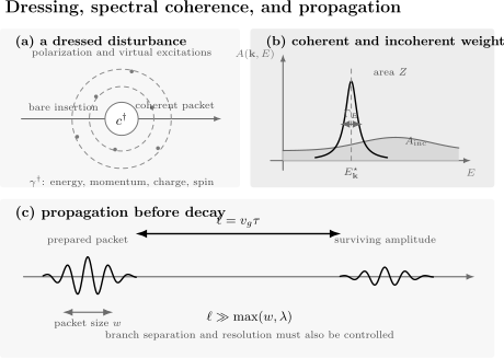
Three complementary quasiparticle tests. Interactions dress a microscopic disturbance into a coherent emergent object. In a chosen operator channel, a narrow peak carries residue $Z$ and width $\Gamma_E$, while the remainder is incoherent spectral weight. In real space, a useful packet propagates over a mean free path $\ell=v_g\tau$ much longer than its wavelength or size.

What the pole does and does not prove

A pole or narrow resonance supports a quasiparticle interpretation in that operator channel. It does not prove that:

• the quasiparticle is weakly dressed;
• the residue is basis independent;
• the peak exhausts the spectral sum rule;
• every observable couples to the branch;
• the same branch is sharp at all momenta;
• a noninteracting thermodynamic formula applies unchanged.

Conversely, absence of weight in one operator does not prove that no excitation exists. A selection rule can make the matrix element vanish.

Stable excitations

If a branch lies below every allowed decay threshold,

$$E_\alpha(\mathbf k) < E_{\mathrm{cont}}^{\min}(\mathbf k),$$

it can be exactly stable at zero temperature. The ideal spectral contribution is then a delta function:

$$A_{\mathrm{coh}} = Z_{\mathbf k} \delta \left( E-E_{\mathbf k} \right).$$

Finite plotting width, experimental resolution, or finite observation time can broaden this line without creating an intrinsic lifetime.

Embedded resonances

If the branch overlaps a multiparticle continuum, decay can be kinematically allowed:

$$\begin{aligned} E_\alpha(\mathbf k) &= \sum_{j=1}^n E_{\beta_j}(\mathbf q_j), \\ \sum_{j=1}^n \mathbf q_j &= \mathbf k+\mathbf G. \end{aligned}$$

Here $\mathbf G$ permits lattice momentum conservation modulo a reciprocal vector. Matrix elements and symmetry determine whether the allowed channel actually produces decay.

Near a threshold, a Lorentzian approximation can fail because the self-energy changes rapidly with energy.

When Is a Quasiparticle Well Defined?

Time-scale criterion

For a gapped or finite-energy excitation, compare the oscillation time

$$t_{\mathrm{osc}} \sim \frac{\hbar}{ \lvert E_{\mathbf k}^\star-E_{\mathrm{ref}}\rvert }$$

with the population lifetime

$$\tau = \frac{\hbar}{\Gamma_E}.$$

A narrow excitation obeys

$$\Gamma_E \ll \lvert E_{\mathbf k}^\star-E_{\mathrm{ref}} \rvert,$$

or equivalently

$$\tau \gg t_{\mathrm{osc}}.$$

Near a gapless point, the denominator tends to zero and this ratio must be interpreted with the appropriate scaling limit. One should compare the width with the local dispersion, mode separation, or experimental frequency scale.

Propagation criterion

The mean free path is

$$\ell_{\mathbf k} = \lvert\mathbf v_g(\mathbf k)\rvert \tau_{\mathbf k}.$$

For a wave packet with spatial size $w$ and wavelength $\lambda$,

$$\ell_{\mathbf k} \gg \max(w,\lambda)$$

means that the packet propagates over many of its own characteristic lengths before decaying.

This is often more intuitive than a pole ratio, especially for acoustic modes.

Branch-separation criterion

If neighboring branches are separated by

$$\Delta_{\mathrm{sep}}(\mathbf k),$$

then

$$\Gamma_E \ll \Delta_{\mathrm{sep}}$$

is needed to assign a unique branch label. Near an avoided crossing, a matrix Green function and coupled-mode analysis may be required.

Spectral-weight criterion

A small residue does not automatically invalidate the quasiparticle. It means that the chosen microscopic operator couples weakly to it. But if:

$$Z\to0, \qquad \Gamma_E \sim \Delta_{\mathrm{sep}},$$

and no alternative operator reveals a sharp mode, particle language is losing predictive value.

Kinematic criterion

A proposed branch must satisfy conservation laws for propagation and decay. Check:

$$\begin{gathered} \text{energy}, \quad \text{momentum}, \quad \text{charge}, \\ \text{spin}, \quad \text{parity}, \quad \text{topological sector}. \end{gathered}$$

An energetically allowed decay can remain forbidden by symmetry. An apparently narrow line can broaden abruptly once a threshold or selection rule changes.

Wave Packets and Semiclassical Motion

Packet construction

A localized quasiparticle packet on one branch is

$$\lvert\Psi_{\mathrm{wp}}\rangle = \sum_{\mathbf k} a(\mathbf k) \gamma_{\mathbf k}^\dagger \lvert\Psi_0\rangle,$$

with $a(\mathbf k)$ concentrated near $\mathbf k_c$.

Expanding the dispersion,

$$\begin{aligned} E(\mathbf k) \simeq{}& E(\mathbf k_c) + \hbar\mathbf v_g \cdot \left( \mathbf k-\mathbf k_c \right) \\ &+ \frac12 \left( \mathbf k-\mathbf k_c \right)_i H_{ij} \left( \mathbf k-\mathbf k_c \right)_j, \end{aligned}$$

where $H_{ij}$ is the Hessian, shows that the linear term translates the packet and the quadratic term spreads it.

Propagation and decay

The packet center moves approximately as

$$\mathbf r_c(t) = \mathbf r_c(0) + \mathbf v_g t$$

before forces and Berry-curvature corrections are included. Its coherent amplitude decays on the pole-amplitude time, while its population decays on the corresponding population time.

The semiclassical picture requires:

• a packet narrow in momentum but localized on relevant macroscopic scales;
• an isolated branch;
• weak variation of parameters across the packet;
• slow external fields;
• scattering rare on the propagation time.

External forces

For a simple band without geometric corrections,

$$\hbar\dot{\mathbf k} = \mathbf F, \qquad \dot{\mathbf r} = \frac{1}{\hbar} \nabla_{\mathbf k}E(\mathbf k).$$

In crystals with nontrivial Berry curvature, anomalous velocity terms can appear. Those band-geometric details belong to Quantum Matter.

Quasiparticles and Collective Modes

Different questions

The quasiparticle question is:

Can an excitation be propagated and scattered as a particle-like object?

The collective-mode question is:

Which coherent macroscopic coordinate oscillates?

The answers can describe the same excitation from different viewpoints.

Operator channels

A microscopic single-particle Green function probes number-changing insertions:

$$c_{\mathbf k}, \qquad c_{\mathbf k}^\dagger.$$

A density or spin response probes number-preserving collective insertions:

$$\rho_{\mathbf q}, \qquad S_{\mathbf q}^\alpha.$$

One mode may appear strongly in one channel and weakly in another. A plasmon is naturally visible in density response. An electron-like quasiparticle is naturally visible in a single-electron spectral function.

Overlap examples

Excitation	Collective origin?	Particle-like quanta?	Natural probe
phonon	yes, lattice displacement	yes	neutron, x-ray, Raman
magnon	yes, spin precession	yes	spin structure factor
plasmon	yes, charge density	yes when underdamped	loss function, optical response
Landau quasiparticle	dressing of fermionic insertion	yes	single-particle spectrum, transport
Bogoliubov quasiparticle	particle–hole mixing	yes	tunneling, photoemission, Bragg
diffusive density mode	yes	generally not ballistic particle-like	hydrodynamic response

Collective Modes develops this boundary systematically through collective coordinates, response eigenvectors, hydrodynamic poles, hybridization, and damping.

Quasiparticle Number and Conserved Charge

Number is often not conserved

For an effective number operator

$$N_{\mathrm{qp}} = \sum_a \gamma_a^\dagger\gamma_a,$$

one can have

$$[H,N_{\mathrm{qp}}] \ne 0.$$

Phonons can be created and annihilated by anharmonic interactions. Magnon number can fail to be exact when spin rotation about the ordering axis is not conserved. Bogoliubov quasiparticle number is not the microscopic atom or electron number.

Conserved microscopic charge

An exact microscopic charge can still be conserved:

$$[H,Q] = 0.$$

A quasiparticle can carry a definite $Q$ charge even when total quasiparticle number changes. In a superconductor, a Bogoliubov excitation is a coherent electron–hole mixture; its charge expectation can depend on momentum even though electric charge conservation holds in the complete gauge-consistent description.

Chemical potential caution

An equilibrium chemical potential is associated with a conserved or externally constrained quantity. One should not add

$$-\mu_{\mathrm{qp}}N_{\mathrm{qp}}$$

merely because a quasiparticle occupation can be counted.

For phonons in ordinary equilibrium,

$$\mu_{\mathrm{ph}} = 0$$

because the material can create and absorb them. Pumping or approximate conservation can produce an effective chemical potential over a restricted time window, but the kinetics must justify it.

Occupation Numbers owns the full operator and ensemble bookkeeping.

Interactions, Scattering, and Kinetics

Golden-rule decay

If a quasiparticle couples to final states through $V_{\mathrm{dec}}$, a weak-coupling decay rate has the schematic form

$$\Gamma_{i\to f}^{\mathrm{rate}} = \frac{2\pi}{\hbar} \sum_f \left| \langle f\lvert V_{\mathrm{dec}} \rvert i\rangle \right|^2 \delta(E_f-E_i).$$

Both matrix elements and final-state phase space matter. A large interaction vertex can produce no decay below threshold; a small vertex can produce strong damping near a large density of states.

Collision integral

When quasiparticles are long lived but not collisionless, their distribution $n_\alpha(\mathbf r,\mathbf k,t)$ can obey a kinetic equation:

$$\frac{\partial n_\alpha}{\partial t} + \dot{\mathbf r} \cdot \nabla_{\mathbf r}n_\alpha + \dot{\mathbf k} \cdot \nabla_{\mathbf k}n_\alpha = I_\alpha[n].$$

The collision integral must include quantum statistics, energy and momentum conservation, and all relevant species.

Collisionless and hydrodynamic regimes

Let $\omega$ be a probe frequency and $\tau_{\mathrm{coll}}$ a collision time.

In the collisionless regime,

$$\omega\tau_{\mathrm{coll}} \gg 1,$$

individual quasiparticle motion can dominate.

In the hydrodynamic regime,

$$\omega\tau_{\mathrm{coll}} \ll 1,$$

local equilibrium and collective conserved-density modes can be more natural.

The existence of quasiparticles and the choice of hydrodynamic variables are related but distinct questions.

Transport lifetime versus spectral lifetime

A single-particle decay rate counts all scattering out of a state. A transport rate weights scattering by its efficiency in relaxing current. For isotropic elastic scattering,

$$\frac{1}{\tau_{\mathrm{tr}}} \propto \int d\Omega\, W(\theta) \left( 1-\cos\theta \right),$$

whereas a single-particle rate is schematically

$$\frac{1}{\tau_{\mathrm{sp}}} \propto \int d\Omega\, W(\theta).$$

Forward scattering can broaden a spectral line while relaxing current inefficiently. Therefore a transport mobility does not directly equal a spectral linewidth.

Representative Quasiparticles

Landau quasiparticles

Near the Fermi surface of a conventional Fermi liquid, interacting fermionic excitations remain in one-to-one correspondence with free-gas particle and hole excitations. They carry the same charge, spin, and momentum labels but have renormalized dispersion and residual interactions.

For excitation energy

$$\varepsilon := E-\mu,$$

the zero-temperature decay rate in a three-dimensional Fermi liquid behaves schematically as

$$\tau^{-1} \propto \varepsilon^2$$

up to model-dependent factors and possible logarithms in lower dimensions. Thus

$$\frac{\hbar/\tau}{\lvert\varepsilon\rvert} \longrightarrow 0$$

as $\varepsilon\to0$, making quasiparticles asymptotically sharp near the Fermi surface.

Bogoliubov quasiparticles in a Bose gas

For a weakly interacting uniform Bose gas,

$$E_k = \sqrt{ \epsilon_k \left( \epsilon_k+2gn_0 \right) }, \qquad \epsilon_k = \frac{\hbar^2k^2}{2m}.$$

At low momentum,

$$E_k \sim \hbar c k,$$

so the quasiparticles are also collective sound quanta. At high momentum,

$$E_k \sim \epsilon_k+gn_0,$$

and they become more particle-like in the microscopic basis.

Weakly Interacting Bose Gas Preview owns depletion, structure factor, and thermodynamics.

Superconducting quasiparticles

In BCS mean-field theory,

$$E_{\mathbf k} = \sqrt{ \xi_{\mathbf k}^2 + \lvert\Delta_{\mathbf k}\rvert^2 }.$$

The excitation is a coherent electron–hole mixture. Near the minimum gap, its charge expectation and coupling to probes depend on coherence factors. Calling it “an electron with a gap” misses that mixing.

Phonons

Phonons as Many-Body Excitations derives the lattice normal modes and their quantization. Their crystal momentum is a mode label conserved modulo reciprocal lattice vectors, not the total mechanical momentum of one moving atom.

At long wavelength an acoustic branch has

$$\omega_\lambda(\mathbf q) \sim c_\lambda \lvert\mathbf q\rvert.$$

Anharmonicity produces phonon–phonon scattering, thermal expansion, and finite lifetimes.

Magnons

Magnons are quanta of spin-wave modes about an ordered magnetic reference state. A one-magnon state is a coherent spin deviation spread over many sites. Its spin quantum number and dispersion depend on the magnetic order and symmetry.

A magnon can decay into multiple magnons if kinematics and interactions allow. Linear spin-wave theory omits those decay processes.

Polarons

A polaron is a mobile impurity or charge carrier dressed by excitations of its environment. The dressing changes:

$$\begin{gathered} \text{energy}, \quad \text{effective mass}, \\ \text{residue}, \quad \text{mobility}, \quad \text{decay thresholds}. \end{gathered}$$

Depending on coupling, a sharp polaron branch can coexist with molecule-like branches and broad continua.

Anyons

Anyons are two-dimensional topological quasiparticles whose worldlines braid. Their identity is encoded by superselection sector, fusion, and braiding data rather than by a bare-particle overlap alone. Anyons and Braiding develops the operational exchange and fusion language, while Fractional Quantum Hall Effect develops the canonical material setting in which fractional charge, braiding-sensitive observables, edge modes, and quantized response meet.

They demonstrate that quasiparticle language is broader than perturbatively dressed microscopic particles.

Breakdown of the Quasiparticle Picture

Width comparable to energy

If

$$\Gamma_E \gtrsim \lvert E^\star-E_{\mathrm{ref}}\rvert,$$

the excitation decays within roughly one oscillation. Assigning a trajectory, occupation, or collision sequence becomes questionable.

For a gapless mode, compare the width to the local dispersion scale rather than dividing by exactly zero.

Overlapping branches

If

$$\Gamma_E \gtrsim \Delta_{\mathrm{sep}},$$

neighboring modes cannot be resolved as independent species. A matrix-valued response, memory kernel, or continuum description may be more faithful.

Branch cuts and continua

An interacting Green function can have a threshold continuum rather than an isolated pole:

$$G^{\mathrm R}(E) \sim \left( E-E_{\mathrm{th}}+i0^+ \right)^{-\alpha}.$$

The corresponding spectral function has a non-Lorentzian edge. Fitting it with a narrow peak plus background can manufacture a quasiparticle that the analytic structure does not contain.

One-dimensional fractionalization

In a generic interacting one-dimensional fermion system, an injected electron can fractionalize into separate collective spin and charge modes. The electron spectral function need not contain a finite-residue Landau pole.

The failure is not absence of useful excitations. It is failure of the electron-like quasiparticle as the low-energy variable. Luttinger Liquid Preview develops the collective replacement, power-law correlations, and spin–charge separation.

Quantum criticality

Near a quantum critical point,

$$\xi\to\infty, \qquad \Delta_{\mathrm{critical}}\to0.$$

Scattering from scale-invariant fluctuations can remove the hierarchy between excitation energy and width. Some critical theories still contain sharp modes; others are dominated by continua. “Critical” does not by itself settle the question.

Confinement

An excitation that is well defined in one regime can become confined in another. If separating two defects costs energy growing with distance,

$$V(r) \sim \sigma r,$$

the isolated defects are not asymptotic quasiparticles. Bound composites can remain well defined.

Orthogonality catastrophe

A sudden local perturbation of a Fermi sea can produce an overlap

$$\left| \langle\Psi_0\vert\Psi_V\rangle \right| \longrightarrow 0$$

as system size grows. Spectral weight is redistributed into many low-energy particle–hole excitations, producing threshold power laws rather than a simple pole.

Overdamped collective response

A response denominator can have the form

$$\chi^{-1}(\mathbf q,\omega) \sim r+cq^2 -i\gamma\omega.$$

When damping dominates the inertial term, the mode relaxes rather than propagates. It is a collective mode, but not necessarily a particle-like quasiparticle.

Strong interaction is not the criterion

Strong microscopic interaction can still produce sharp low-energy quasiparticles, as in a conventional Fermi liquid. Weak coupling can fail when infrared phase space, nesting, dimensionality, or a degeneracy makes perturbations singular.

The correct question is: Does the chosen low-energy branch remain isolated, coherent, and long lived?

Temperature and Nonequilibrium

Thermal broadening

At nonzero temperature, thermally occupied excitations open additional scattering channels:

$$\Gamma_E = \Gamma_E(\mathbf k,T).$$

In a Fermi liquid near the Fermi surface,

$$\Gamma_E \propto \varepsilon^2 + \left( \pi k_{\mathrm B}T \right)^2$$

schematically. The coefficient and logarithmic corrections are system dependent.

A branch sharp at $T=0$ can become overdamped above a crossover temperature without a thermodynamic phase transition.

State dependence

Quasiparticles are defined relative to a background state:

$$\lvert\Psi_0\rangle, \qquad \rho_\beta, \qquad \rho(t).$$

Changing density, order, temperature, or drive changes the dressing and available decay channels. The same microscopic operator can create different effective excitations in different phases.

Pumped quasiparticles

After a drive, a distribution of quasiparticles may be useful even when it is not thermal. One must then specify:

• preparation protocol;
• dephasing and collision times;
• whether the instantaneous spectrum changes;
• whether quasiparticle number is approximately conserved;
• which kinetic equation applies.

Fitting a transient occupation to a thermal Bose or Fermi function does not by itself establish equilibrium.

Prethermal regimes

A driven or weakly nonintegrable system can exhibit a long prethermal window in which approximate quasiparticles are conserved:

$$t_{\mathrm{micro}} \ll t \ll t_{\mathrm{thermal}}.$$

The effective description can be accurate in this window even though it fails asymptotically.

How Quasiparticles Are Observed

Operator-resolved spectra

No experiment measures “the quasiparticle” without a coupling operator. A measured intensity has the schematic form

$$\begin{aligned} I &\sim \lvert M_{\mathrm{probe}}\rvert^2 \times \text{occupation factor} \\ &\quad\times \text{spectral function} \ast \text{resolution}. \end{aligned}$$

The operator determines which quantum numbers and matrix elements are visible.

Single-particle probes

Photoemission, inverse photoemission, tunneling, and radio-frequency spectroscopy can probe addition or removal spectra. They are natural for electron-like, atom-like, hole-like, and Bogoliubov quasiparticles.

The observed peak includes:

• intrinsic spectral weight;
• probe matrix elements;
• occupation restrictions;
• final-state effects;
• energy and momentum resolution.

Scattering probes

Neutron, x-ray, light, and Bragg scattering probe density, spin, displacement, or other number-preserving correlations. They naturally reveal collective quasiparticles such as phonons and magnons.

Structure Factors owns the momentum–energy transfer conventions.

Transport

Electrical, thermal, and spin transport can infer quasiparticle velocities, densities, charges, and scattering times. The inference is model dependent because vertex corrections and conservation laws distinguish transport from single-particle decay.

Thermodynamics

Low-temperature heat capacity, susceptibility, and compressibility constrain the density of low-energy states and effective interactions. They can support a quasiparticle description but rarely identify the full spectral function alone.

A convergence standard

A strong identification combines:

$$\begin{gathered} \text{continuous dispersion}, \\ \text{symmetry-consistent quantum numbers}, \\ \text{controlled linewidth}, \\ \text{sum-rule-compatible weight}, \\ \text{response across more than one} \\ \text{observable}. \end{gathered}$$

One fitted peak is evidence, not a complete ontology.

A Practical Quasiparticle Checklist

Define the reference state

State the phase, density, temperature, fields, and boundary conditions. A quasiparticle is an excitation of that background.

Name the creation channel

Specify the microscopic operator or response field:

$$c_{\mathbf k}^\dagger, \quad \rho_{\mathbf q}, \quad S_{\mathbf q}^\alpha, \quad u_{\mathbf q\lambda}.$$

This determines selection rules and residue.

Trace a branch

Identify a continuous $E_\alpha(\mathbf k)$ across neighboring momenta. A collection of unrelated maxima is not automatically one quasiparticle branch.

Resolve the width

Separate:

• intrinsic damping;
• instrumental resolution;
• finite-time or finite-size broadening;
• disorder and inhomogeneous broadening;
• artificial numerical kernels.

Then compare $\Gamma_E$ with energy, branch separation, and thresholds.

Check weight and sum rules

Verify that coherent and incoherent pieces respect the relevant normalization:

$$Z + \int dE\, A_{\mathrm{inc}}(E) = \text{channel sum rule}.$$

The right-hand side depends on operator normalization and can include multiple coherent branches.

Identify decay channels

List all states satisfying energy, momentum, and quantum-number conservation. Track where thresholds open.

State the effective cutoff

Give the domain

$$\mathcal R_{\mathrm{qp}} = \left\{ (\mathbf k,E,T,\ldots): \text{criteria satisfied} \right\}.$$

The boundary of this region is as important as the best-fit parameters inside it.

Validate another observable

Compare the inferred branch with an independent probe, thermodynamic coefficient, or controlled numerical calculation. Agreement tests the effective interpretation rather than only the fitting function.

Common Mistakes

Treating a quasiparticle as a hidden microscopic constituent

A phonon is not one atom, and a magnon is not one preexisting spin bead. They are quantized disturbances of an interacting background.

Calling every exact eigenstate a quasiparticle

Exact stationarity is not particle-like organization. A dense many-body eigenstate can have no useful dispersion, local creation operator, or dilute-gas interpretation.

Calling every spectral maximum a quasiparticle

Thresholds, van Hove features, overlapping lines, and resolution kernels can create maxima without isolated poles.

Using peak height as residue

Residue is integrated coherent weight in a normalized channel. Peak height also depends on width, background, matrix elements, and resolution.

Equating spectral and transport lifetimes

Forward scattering can strongly affect one and weakly affect the other. State which correlator or relaxation process defines the time.

Requiring quasiparticle number conservation

Many useful quasiparticles can be created and destroyed. Conserved charge and quasiparticle count are different operators.

Assuming weak interaction guarantees sharp particles

Low dimension, degeneracy, resonant phase space, or infrared singularities can destroy a naive perturbative particle picture.

Assuming strong interaction forbids quasiparticles

Strongly interacting systems can flow to low-energy fixed points with long-lived emergent excitations.

Confusing collective with non-particle-like

Phonons and magnons are collective in construction and quasiparticle-like after quantization. Diffusive modes are collective but generally not ballistic quasiparticles.

Extending a low-energy branch beyond its cutoff

An effective dispersion can merge into a continuum, cross another branch, or reach lattice-scale physics. Extrapolation beyond the validated regime is not a prediction of the quasiparticle theory.

Exercises

Exercise 1: Classify the excitation

For each description, state which labels apply: microscopic particle, exact eigenexcitation, normal mode, quasiparticle, collective mode, or resonance. More than one label can apply.

1. One quantum of a harmonic crystal displacement mode.
2. An arbitrary highly excited eigenstate of a finite interacting spin chain.
3. A narrow finite-lifetime electron-addition peak in a metal.
4. A diffusive conserved-density pole.
5. A stable exciton below the electron–hole continuum.

Solution

1. A phonon is a normal-mode quantum, a collective mode, an exact eigenexcitation of the harmonic approximation, and a quasiparticle. Anharmonicity makes it metastable.
2. It is an exact eigenexcitation. No other label follows without additional structure.
3. It is a resonance and a quasiparticle. It is not a new microscopic particle.
4. It is a collective mode, but generally not a ballistic particle-like quasiparticle because its dynamics is relaxational.
5. It is a bound composite, an exact stable excitation in the ideal closed system, and a quasiparticle below breakup threshold.

The exercise shows why the categories overlap and why each word answers a different question.

Exercise 2: Pole parameters from a self-energy

Suppose

$$\Sigma^{\mathrm R}(E) = -\lambda E - i\gamma_0, \qquad \lambda>0,$$

near a reference level $\xi$. Find the renormalized energy, residue, intrinsic HWHM, spectral FWHM, and population lifetime.

Solution

The pole equation is

$$E^\star-\xi+\lambda E^\star = 0,$$

so

$$E^\star = \frac{\xi}{1+\lambda}.$$

The residue is

$$Z = \frac{1}{1+\lambda}.$$

Thus $0<Z<1$: the coherent pole carries only part of the unit spectral weight. A complete causal self-energy must supply the remaining weight through its full frequency dependence and the corresponding incoherent spectrum.

The HWHM is

$$\gamma = -Z\Sigma'' = Z\gamma_0.$$

Therefore

$$\Gamma_E = 2Z\gamma_0$$

and, for the population convention,

$$\tau_{\mathrm{pop}} = \frac{\hbar}{2Z\gamma_0}.$$

This example also warns that a local pole expansion fixes the neighborhood of one peak, not the complete spectral function.

Exercise 3: Coherent weight

Show that

$$A_{\mathrm{coh}}(E) = \frac{Z}{\pi} \frac{\gamma}{ (E-E^\star)^2+\gamma^2 }$$

has integrated area $Z$. What happens to the line as $\gamma\to0^+$?

Solution

Set

$$x = \frac{E-E^\star}{\gamma}, \qquad dE = \gamma\,dx.$$

Then

$$\begin{aligned} \int_{-\infty}^{\infty} dE\, A_{\mathrm{coh}}(E) &= \frac{Z}{\pi} \int_{-\infty}^{\infty} \frac{dx}{1+x^2} \\ &= Z. \end{aligned}$$

As $\gamma\to0^+$,

$$\frac{1}{\pi} \frac{\gamma}{ (E-E^\star)^2+\gamma^2 } \longrightarrow \delta(E-E^\star)$$

in the distributional sense. The peak height diverges while the area remains $Z$. This is why peak height is not residue.

Exercise 4: Propagation quality

A quasiparticle has group velocity

$$v_g = 2.0\times10^5\ \mathrm{m\,s^{-1}},$$

population lifetime

$$\tau = 0.50\ \mathrm{ps},$$

and wavelength

$$\lambda = 5.0\ \mathrm{nm}.$$

Compute its mean free path and the number of wavelengths traversed before decay.

Solution

The mean free path is

$$\begin{aligned} \ell &= v_g\tau \\ &= \left( 2.0\times10^5\ \mathrm{m\,s^{-1}} \right) \left( 0.50\times10^{-12}\ \mathrm s \right) \\ &= 1.0\times10^{-7}\ \mathrm m \\ &= 100\ \mathrm{nm}. \end{aligned}$$

Thus

$$\frac{\ell}{\lambda} = \frac{100\ \mathrm{nm}}{5.0\ \mathrm{nm}} = 20.$$

The packet travels about twenty wavelengths, which supports a propagating particle-like interpretation if branch separation and packet-spreading criteria are also satisfied.

Exercise 5: Quasiparticle vacuum

For a bosonic Bogoliubov transformation

$$a = u\gamma + v^*\gamma^\dagger, \qquad \lvert u\rvert^2-\lvert v\rvert^2=1,$$

let

$$\gamma\lvert0_\gamma\rangle = 0.$$

Compute the microscopic occupation $\langle a^\dagger a\rangle$.

Solution

The adjoint is

$$a^\dagger = u^*\gamma^\dagger + v\gamma.$$

Therefore

$$\begin{aligned} a^\dagger a = {}& \lvert u\rvert^2 \gamma^\dagger\gamma + u^*v^* \gamma^\dagger\gamma^\dagger \\ & + vu \gamma\gamma + \lvert v\rvert^2 \gamma\gamma^\dagger. \end{aligned}$$

Only the last term survives in the quasiparticle vacuum:

$$\langle0_\gamma\lvert a^\dagger a \rvert0_\gamma\rangle = \lvert v\rvert^2.$$

Zero quasiparticles does not mean zero microscopic particles. The background and operator basis must be named.

Exercise 6: Number versus charge

An anharmonic phonon Hamiltonian contains

$$H_3 \sim \sum_{123} g_{123} \left( b_1^\dagger b_2 b_3 + \mathrm{h.c.} \right).$$

Does total phonon number commute with $H_3$? Does this imply violation of energy or microscopic atom-number conservation?

Solution

For

$$N_{\mathrm{ph}} = \sum_i b_i^\dagger b_i,$$

the term $b_1^\dagger b_2b_3$ creates one phonon and annihilates two, changing $N_{\mathrm{ph}}$ by $-1$. Hence

$$[H_3,N_{\mathrm{ph}}] \ne 0.$$

This does not violate energy conservation. A real decay occurs only when the participating mode energies satisfy the relevant conservation condition, broadened as appropriate in a finite-time process.

It also does not violate microscopic atom-number conservation. Phonons are quanta of displacement normal modes, not atoms. Their number is an effective excitation count.

Exercise 7: Operator-dependent residue

Let an exact normalized excitation be

$$\lvert\Phi\rangle = \frac{1}{\sqrt5} c_1^\dagger\lvert\Psi_0\rangle + \frac{2}{\sqrt5} c_2^\dagger\lvert\Psi_0\rangle,$$

where the two created states are orthonormal. Find its pole residue in the $c_1^\dagger$ and $c_2^\dagger$ channels. Can the excitation’s existence depend on which channel is chosen?

Solution

The overlap amplitudes are

$$\langle\Phi\lvert c_1^\dagger \rvert\Psi_0\rangle = \frac{1}{\sqrt5},$$

and

$$\langle\Phi\lvert c_2^\dagger \rvert\Psi_0\rangle = \frac{2}{\sqrt5}.$$

The residues are the squared magnitudes:

$$Z_1 = \frac15, \qquad Z_2 = \frac45.$$

The excitation is one exact state of the Hamiltonian. Its existence does not depend on the probe. Its visibility and spectral weight do depend on the operator channel.

Exercise 8: Audit a quasiparticle claim

A numerical spectrum on one finite cluster shows a broad maximum at energy $E_0$. The calculation used an artificial Lorentzian broadening $\eta=0.2J$. A fit returns FWHM $0.24J$, and the authors report an intrinsic lifetime $\hbar/(0.24J)$.

What is wrong with the claim, and what additional evidence is needed?

Solution

The displayed width is dominated by a numerical kernel whose scale is already comparable to the fitted FWHM. It cannot be interpreted directly as intrinsic decay.

In a finite closed system, the exact spectrum is a set of delta lines. A broad maximum can represent:

• one line broadened by $\eta$;
• several unresolved lines;
• the finite-size precursor of a continuum;
• a threshold or density-of-states feature;
• a true resonance only after an appropriate thermodynamic limit.

A responsible analysis should:

1. repeat the calculation for several $\eta$ values;
2. examine raw line positions and weights;
3. scale system size and boundary conditions;
4. test whether a continuous branch exists across momentum;
5. compare the candidate width with level spacing and resolution;
6. identify allowed decay channels in the infinite system;
7. verify residue and sum-rule stability;
8. use real-time decay or another independent method when possible.

Only an intrinsic width remaining after these controls can support a lifetime estimate.

Key Takeaways

• A quasiparticle is an emergent particle-like excitation, not usually an extra microscopic constituent.
• Its definition requires a background state, energy–momentum regime, operator channel, and accuracy criterion.
• Particle-like data include dispersion, quantum numbers, statistics, residue, lifetime, and residual interactions.
• Exact eigenstate, normal mode, resonance, collective mode, and quasiparticle are overlapping but distinct labels.
• Quasiparticles arise through normal-mode quantization, Bogoliubov mixing, adiabatic dressing, binding, holes, and topological sectors.
• The leading effective Hamiltonian is approximately additive, but residual interactions and decay vertices remain.
• A narrow Green-function pole gives a compact diagnostic, while residue remains operator dependent and incoherent weight remains physical.
• The controlled regime requires width small compared with energy, branch separation, or the relevant local dispersion scale.
• In real space, a useful packet has mean free path $\ell=v_g\tau$ much larger than its own wavelength or size.
• Collective modes can have quasiparticle quanta; collective origin and particle-like propagation are not opposites.
• Quasiparticle number need not be conserved even when exact microscopic charges are.
• Strong interactions do not automatically destroy quasiparticles, and weak interactions do not guarantee them.
• Broad continua, branch cuts, criticality, fractionalization, confinement, and overdamping can invalidate the particle picture.
• Experimental identification requires operator-aware spectra, resolution control, sum rules, threshold analysis, and independent cross-checks.

Further Reading

• For exact number-changing correlators, see Green Functions in Many-Body QM.
• For peak, residue, width, continuum, and resolution conventions, see Spectral Functions.
• For low-energy projection and matching, see Effective Hamiltonians in Many-Body Systems.
• For canonical bosonic mode mixing, see Bogoliubov Theory.
• For particle and quasiparticle counting, see Occupation Numbers.
• For a materials-facing learning path, see the Condensed Matter Roadmap.

References

• L. D. Landau, “The Theory of a Fermi Liquid”, Soviet Physics JETP 3, 920–925, 1957; Russian original received in 1956.
• H. Lehmann, “Über Eigenschaften von Ausbreitungsfunktionen und Renormierungskonstanten quantisierter Felder”, Il Nuovo Cimento 11, 342–357, 1954.
• F. J. Dyson, “The Radiation Theories of Tomonaga, Schwinger, and Feynman”, Physical Review 75, 486–502, 1949.
• J. J. Quinn and R. A. Ferrell, “Electron Self-Energy Approach to Correlation in a Degenerate Electron Gas”, Physical Review 112, 812–827, 1958.
• J. M. Luttinger, “Analytic Properties of Single-Particle Propagators for Many-Fermion Systems”, Physical Review 121, 942–949, 1961.
• N. N. Bogoliubov, “On the Theory of Superfluidity,” Journal of Physics (USSR) 11, 23–32, 1947.
• J. Bardeen, L. N. Cooper, and J. R. Schrieffer, “Theory of Superconductivity”, Physical Review 108, 1175–1204, 1957.
• Y. Nambu, “Quasi-Particles and Gauge Invariance in the Theory of Superconductivity”, Physical Review 117, 648–663, 1960.
• P. W. Anderson, “More Is Different”, Science 177, 393–396, 1972.
• R. B. Laughlin and D. Pines, “The Theory of Everything”, Proceedings of the National Academy of Sciences 97, 28–31, 2000.
• A. Damascelli, Z. Hussain, and Z.-X. Shen, “Angle-Resolved Photoemission Studies of the Cuprate Superconductors”, Reviews of Modern Physics 75, 473–541, 2003.
• A. L. Fetter and J. D. Walecka, Quantum Theory of Many-Particle Systems, Dover, 2003.
• G. D. Mahan, Many-Particle Physics, 3rd ed., Springer, 2000.
• P. Coleman, Introduction to Many-Body Physics, Cambridge University Press, 2015.
• D. Pines and P. Nozières, The Theory of Quantum Liquids, Volume I: Normal Fermi Liquids, CRC Press, 2018 reissue.
• G. Baym and C. Pethick, Landau Fermi-Liquid Theory, Wiley-VCH, 1991.
• A. A. Abrikosov, L. P. Gorkov, and I. E. Dzyaloshinski, Methods of Quantum Field Theory in Statistical Physics, Dover, 1975.
• A. Altland and B. Simons, Condensed Matter Field Theory, 2nd ed., Cambridge University Press, 2010.