Bogoliubov Quasiparticles

A Bogoliubov quasiparticle is a positive-frequency canonical normal excitation whose annihilation operator is a linear combination of the original annihilation and creation operators. The mixing is defined relative to a condensate, paired state, ordered texture, or other reference background. It occurs when the quadratic fluctuation Hamiltonian contains anomalous terms that create or annihilate pairs of the original modes.

For one translation-invariant pair of momenta, the schematic operator is

$$\eta_{\mathbf k} := u_{\mathbf k}a_{\mathbf k} + v_{\mathbf k}a_{-\mathbf k}^\dagger.$$

The coefficient $u_{\mathbf k}$ is conventionally called the particle amplitude and $v_{\mathbf k}$ the hole amplitude. This language must be interpreted carefully:

• for a fermion paired across a Fermi surface, the hole component is literally the removal of an occupied fermionic mode;
• for a weakly interacting Bose condensate, the “hole” component is the negative-frequency creation partner in Nambu space, not a vacancy inside a filled Bose sea;
• in either case, the two terms carry the same conserved momentum and other unbroken quantum numbers, so they may form one normal mode;
• the amplitudes control both the composition of the excitation and the matrix element seen by a probe.

The transformation does more than change basis. It changes which state is called the vacuum. A Bogoliubov vacuum is annihilated by every $\eta_{\mathbf k}$ but generally contains pairs of the original particles. One quasiparticle therefore need not equal one microscopic particle, one unit of microscopic charge, or one local disturbance.

Scope and Canonical Ownership

This page owns the excitation-centered interpretation:

• why anomalous quadratic terms mix creation and annihilation operators;
• the definition of a positive-frequency Bogoliubov quasiparticle;
• Nambu doubling and the distinction between a physical branch and its redundant partner;
• bosonic paraunitary versus fermionic unitary normalization;
• hyperbolic squeezing versus compact particle–hole rotation;
• the structure of bosonic squeezed vacua and fermionic paired vacua;
• momentum, spin, parity, and microscopic-number expectations;
• coherence factors in single-particle and collective probes;
• weak-Bose-gas and BCS applications as contrasting physical realizations;
• thermal occupations, interactions, lifetime, stability, and breakdown;
• the relation to positive- and negative-frequency mode decompositions in quantum field theory.

Neighboring pages retain more specialized ownership:

• Quasiparticles Overview owns the general criteria of dispersion, residue, lifetime, wave-packet propagation, and quasiparticle breakdown.
• Bogoliubov Theory owns the full bosonic Nambu bookkeeping, paraunitary algorithm, generalized eigenproblem, zero modes, and stability diagnostics.
• Weakly Interacting Bose Gas Preview owns the dilute-gas equation of state, depletion coefficient, Lee–Huang–Yang correction, and superfluidity.
• BCS Mean-Field Theory owns the Cooper instability, mean-field decoupling, self-consistent gap and number equations, and superconducting thermodynamics.
• Squeezed States as Entangled Modes owns the quantum-information structure of bosonic squeezing and continuous-variable entanglement.
• Spectral Functions owns exact Lehmann normalization, self-energy broadening, line shapes, sum rules, and experimental resolution.
• Structure Factors owns density and spin response conventions, detailed balance, and scattering normalization.

The page does not redo every diagonalization or self-consistency calculation. It asks what the resulting operators create, what quantum numbers those excitations have, what a probe sees, and when the quasiparticle interpretation is justified.

When those excitations enter a material superfluid or superconducting claim, use Superfluidity and Superconductivity to choose the phase and response branch; this page retains operator interpretation and physical branch counting.

The Defining Eigenoperator

Positive-frequency excitation

Let $K$ denote the generator used for the stationary problem. It may be $H$, a grand-canonical operator $H-\mu N$, or a rotating-frame generator. A normalized quasiparticle creator $\eta_\nu^\dagger$ satisfies

$$\left[ K_2, \eta_\nu^\dagger \right] := E_\nu \eta_\nu^\dagger, \qquad E_\nu>0,$$

for the quadratic Hamiltonian $K_2$.

The quasiparticle vacuum obeys

$$\eta_\nu \lvert0_\eta\rangle := 0$$

for every positive-frequency mode. Then

$$\lvert1_\nu\rangle := \eta_\nu^\dagger \lvert0_\eta\rangle$$

has excitation energy $E_\nu$ within the quadratic theory.

The diagonal form is

$$K_2 := K_{\mathrm{vac}} + \sum_{\nu>0} E_\nu \eta_\nu^\dagger\eta_\nu.$$

Only positive-frequency modes are counted as independent annihilation operators. Their negative-frequency Nambu partners reconstruct the adjoint creation operators; they are not extra negative-energy particles.

Statistics are preserved

A canonical transformation does not turn bosons into fermions or fermions into bosons. For bosonic modes,

$$\left[ \eta_\mu,\eta_\nu^\dagger \right] := \delta_{\mu\nu}.$$

For fermionic modes,

$$\left\{ \eta_\mu,\eta_\nu^\dagger \right\} := \delta_{\mu\nu}.$$

Thus a bosonic Bogoliubov quasiparticle can occupy one mode arbitrarily many times within the approximation, while a fermionic Bogoliubov mode has occupation zero or one.

Exact eigenstate versus quadratic excitation

The eigenoperator equation is exact for $K_2$, not automatically for the microscopic interacting Hamiltonian. If

$$K := K_2 + K_{\mathrm{int}},$$

then generally

$$\left[ K, \eta_\nu^\dagger \right] \neq E_\nu\eta_\nu^\dagger.$$

The omitted cubic and higher terms scatter quasiparticles, shift their energies, and may give them finite lifetimes. “Bogoliubov quasiparticle” therefore names both a precise harmonic excitation and, when interactions are weak enough, the continuously connected resonance in the full system.

Why Mixing Appears

Expansion around a background

Suppose a field or mode has a nonzero reference amplitude:

$$\hat\psi := \Phi + \delta\hat\psi.$$

Expanding an interacting Hamiltonian gives

$$K := K^{[0]} + K^{[1]} + K^{[2]} + K^{[3]} + \cdots.$$

Stationarity of the chosen background requires

$$K^{[1]} := 0.$$

The quadratic term can contain both normal bilinears,

$$a_i^\dagger A_{ij}a_j,$$

and anomalous bilinears,

$$\frac12 \left( a_i^\dagger B_{ij}a_j^\dagger + \mathrm{h.c.} \right).$$

The anomalous terms say that the reference background can exchange pairs with the fluctuation sector. An operator $a_i^\dagger$ alone is then not a normal excitation because its equation of motion couples to annihilation operators.

Exact symmetry need not be absent

The microscopic Hamiltonian may conserve particle number exactly even when the quadratic representation does not. In a symmetry-breaking treatment:

• a Bose condensate amplitude replaces one macroscopically occupied operator by a complex number;
• a BCS pair field replaces pair scattering by an anomalous mean field;
• the quadratic fluctuation Hamiltonian is organized relative to a phase-selected reference;
• the condensate or pair background supplies the number exchanged by anomalous terms.

Number-conserving formulations can recover the same positive-frequency spectrum while keeping exact $N$. The anomalous representation is a calculational organization, not proof that the microscopic Hamiltonian violates its symmetry.

Ordinary basis rotations are insufficient

An ordinary one-particle rotation has the form

$$\widetilde a_\mu := \sum_i U_{i\mu}^* a_i$$

and never mixes $a$ with $a^\dagger$. It diagonalizes a number-conserving quadratic form. Once $B\neq0$, the normal mode requires the enlarged transformation

$$\eta_\nu := \sum_i \left( u_{i\nu}^*a_i + v_{i\nu}^*a_i^\dagger \right).$$

This is a canonical transformation in phase space or Nambu space, not merely a rotation among one-particle orbitals.

Nambu Space Without Double Counting

Doubled vector

For $M$ original modes, define

$$\Psi := \begin{pmatrix} \mathbf a \\ \mathbf a^\dagger \end{pmatrix}.$$

The quadratic Hamiltonian can be written

$$K_2 := \frac12 \Psi^\dagger \mathcal H_{\mathrm N} \Psi + C.$$

The $2M$ components are not $2M$ independent particles. The lower half is fixed as the adjoint of the upper half. The factor $1/2$ and constant $C$ repair the double counting and operator reordering introduced by this notation.

Partner modes

If

$$w_\nu := \begin{pmatrix} \mathbf u_\nu \\ \mathbf v_\nu \end{pmatrix}$$

represents a positive-frequency mode, Nambu conjugation constructs a partner of schematic form

$$\overline w_\nu := \begin{pmatrix} \mathbf v_\nu^* \\ \mathbf u_\nu^* \end{pmatrix}.$$

The partner appears at $-E_\nu$ in the doubled eigenproblem. It supplies $\eta_\nu^\dagger$, not a second annihilator with negative physical energy.

The exact conjugation matrix and signs depend on the bosonic or fermionic convention and on spin or orbital labels. The invariant rule is to count one complete positive-frequency, positive-norm set.

Bosonic Canonical Geometry

Indefinite metric

For bosons, the Nambu commutators are encoded by

$$\Sigma_z := \begin{pmatrix} I&0 \\ 0&-I \end{pmatrix}.$$

A transformation $\Psi=T\Gamma$ preserves commutators when

$$T^\dagger \Sigma_z T := \Sigma_z.$$

This is paraunitarity. The positive-frequency mode normalization is

$$w_\nu^\dagger \Sigma_z w_\nu := 1.$$

The dynamical eigenproblem is

$$\Sigma_z \mathcal H_{\mathrm N} w_\nu := E_\nu w_\nu,$$

not ordinary unitary diagonalization of $\mathcal H_{\mathrm N}$ alone.

One opposite-momentum block

Consider

$$\begin{aligned} K_{\mathrm B} := A \Big( & a_{\mathbf k}^\dagger a_{\mathbf k} + a_{-\mathbf k}^\dagger a_{-\mathbf k} \Big) \\ &+ B \left( a_{\mathbf k}^\dagger a_{-\mathbf k}^\dagger + a_{\mathbf k}a_{-\mathbf k} \right), \end{aligned}$$

with real $A$ and $B$. Use

$$\begin{aligned} a_{\mathbf k} &:= u b_{\mathbf k} - v b_{-\mathbf k}^\dagger, \\ a_{-\mathbf k} &:= u b_{-\mathbf k} - v b_{\mathbf k}^\dagger. \end{aligned}$$

Commutator preservation requires

$$u^2-v^2 := 1.$$

Write

$$u := \cosh r, \qquad v := \sinh r.$$

The anomalous term vanishes when

$$\tanh(2r) := \frac BA.$$

For

$$A>\lvert B\rvert,$$

the positive energy is

$$E := \sqrt{ A^2-B^2 }.$$

The coherence factors may be chosen as

$$\begin{aligned} u^2 &:= \frac12 \left( \frac AE+1 \right), \\ v^2 &:= \frac12 \left( \frac AE-1 \right), \\ uv &:= \frac{B}{2E}. \end{aligned}$$

As $A\to\lvert B\rvert^+$, the mode softens and $u,v$ grow. Their difference remains constrained while their Euclidean norm need not.

Stability meaning

If

$$A<\lvert B\rvert,$$

then $E$ is imaginary. The assumed background has an exponentially growing fluctuation; there is no stable bosonic quasiparticle with that frequency.

A real-looking eigenvalue is not the only check in a multimode problem. One must also verify the paraunitary norm, completeness, energy boundedness, and treatment of exact zero modes. The general algorithm belongs to Bogoliubov Theory.

Fermionic Canonical Geometry

Compact normalization

For fermions, anticommutator preservation gives an ordinary unitary condition in each independent Nambu block. A paired spin block may be written

$$\begin{pmatrix} \gamma_{\mathbf k\uparrow} \\ \gamma_{-\mathbf k\downarrow}^\dagger \end{pmatrix} := \begin{pmatrix} u_{\mathbf k} & -v_{\mathbf k} \\ v_{\mathbf k}^* & u_{\mathbf k} \end{pmatrix} \begin{pmatrix} c_{\mathbf k\uparrow} \\ c_{-\mathbf k\downarrow}^\dagger \end{pmatrix}.$$

The normalization is

$$u_{\mathbf k}^2 + \lvert v_{\mathbf k}\rvert^2 := 1.$$

One may parameterize

$$u_{\mathbf k} := \cos\theta_{\mathbf k}, \qquad \lvert v_{\mathbf k}\rvert := \sin\theta_{\mathbf k}.$$

Unlike bosonic squeezing, fermionic particle–hole rotation is compact because Pauli exclusion bounds each occupation.

Paired two-by-two block

Choose the Hermitian matrix

$$h_{\mathbf k} := \begin{pmatrix} \xi_{\mathbf k} & -\Delta_{\mathbf k} \\ -\Delta_{\mathbf k}^* & -\xi_{\mathbf k} \end{pmatrix},$$

where $\xi_{\mathbf k}$ is measured from the chemical potential. Its eigenvalues are

$$\pm E_{\mathbf k},$$

with

$$E_{\mathbf k} := \sqrt{ \xi_{\mathbf k}^2 + \lvert\Delta_{\mathbf k}\rvert^2 }.$$

The positive-branch coherence factors can be chosen as

$$\begin{aligned} u_{\mathbf k}^2 &:= \frac12 \left( 1 + \frac{ \xi_{\mathbf k} }{ E_{\mathbf k} } \right), \\ \lvert v_{\mathbf k}\rvert^2 &:= \frac12 \left( 1 - \frac{ \xi_{\mathbf k} }{ E_{\mathbf k} } \right). \end{aligned}$$

Their relative phase follows the phase of $\Delta_{\mathbf k}$. For example,

$$u_{\mathbf k}v_{\mathbf k} := \frac{ \Delta_{\mathbf k} }{ 2E_{\mathbf k} }$$

in a compatible convention.

Far above the Fermi surface, $u_{\mathbf k}^2\to1$ and the quasiparticle is particle-like. Far below it, $\lvert v_{\mathbf k}\rvert^2\to1$ and the positive-energy excitation is hole-like. At $\xi_{\mathbf k}=0$, both weights are $1/2$: pairing has turned the normal-state crossing into an avoided crossing.

Reality does not prove saddle stability

The finite fermionic BdG matrix is Hermitian, so its eigenvalues are real. That does not prove that the assumed pair field minimizes the original interacting problem. The gap must be found self-consistently and tested against competing saddles, phase fluctuations, number constraints, and interaction corrections.

Bosonic complex frequencies diagnose dynamical instability directly. Fermionic mean-field failure usually appears instead through an unfavorable free energy, a missing self-consistent solution, a soft collective fluctuation, or strong corrections beyond the quadratic saddle.

Bosons and Fermions Side by Side

Feature	Bosonic mode	Fermionic mode
Algebra preserved	Commutator	Anticommutator
Scalar norm	$	u
Geometry	Hyperbolic	Circular
Nambu map	Paraunitary	Unitary in paired block
Vacuum	Squeezed pair state	Empty–paired state
Mode occupation	Unbounded	Zero or one
Soft-mode warning	$u,v$ may diverge; frequency may be complex	Coefficients stay bounded
Exact residual	Model dependent	Fermion parity

The shared name “Bogoliubov transformation” means that the appropriate canonical algebra is preserved. It does not mean that the bosonic and fermionic eigenproblems, norms, stability criteria, or vacuum structures are interchangeable.

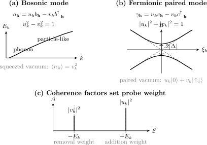
Bosonic mixing is hyperbolic and produces a squeezed vacuum; fermionic mixing is unitary and produces an empty–paired superposition. In a fermionic single-particle spectrum, the coherence factors redistribute weight between addition and removal peaks.

The Quasiparticle Vacua

Bosonic two-mode squeezed vacuum

The inverse of the bosonic transformation is

$$b_{\mathbf k} := u a_{\mathbf k} + v a_{-\mathbf k}^\dagger.$$

The state satisfying

$$b_{\mathbf k} \lvert0_b\rangle := 0$$

for both members of the pair is

$$\lvert0_b\rangle := \frac1u \sum_{n=0}^{\infty} \left( - \frac vu \right)^n \lvert n_{\mathbf k},n_{-\mathbf k}\rangle.$$

Its contractions are

$$\begin{aligned} \left\langle a_{\mathbf k}^\dagger a_{\mathbf k} \right\rangle_b &:= v^2, \\ \left\langle a_{\mathbf k}a_{-\mathbf k} \right\rangle_b &:= -uv. \end{aligned}$$

The vacuum has no $b$ quasiparticles but contains correlated pairs of $a$ particles. Tracing out one momentum gives a geometric occupation distribution, which is why the two modes are entangled.

Fermionic BCS pair vacuum

For one time-reversed pair, the quasiparticle vacuum is

$$\lvert\mathrm{BCS}\rangle_{\mathbf k} := u_{\mathbf k} \lvert0\rangle + v_{\mathbf k} \lvert \mathbf k\uparrow, -\mathbf k\downarrow \rangle.$$

The series stops after one pair because Pauli exclusion forbids a second occupation of either spin orbital. The full mean-field state is the product

$$\lvert\mathrm{BCS}\rangle := \prod_{\mathbf k} \left( u_{\mathbf k} + v_{\mathbf k} c_{\mathbf k\uparrow}^\dagger c_{-\mathbf k\downarrow}^\dagger \right) \lvert0\rangle.$$

Its contractions include

$$\begin{aligned} \left\langle c_{\mathbf k\uparrow}^\dagger c_{\mathbf k\uparrow} \right\rangle &:= \lvert v_{\mathbf k}\rvert^2, \\ \left\langle c_{-\mathbf k\downarrow} c_{\mathbf k\uparrow} \right\rangle &:= u_{\mathbf k}v_{\mathbf k}. \end{aligned}$$

The state has even fermion parity but, before number projection, is a coherent superposition of different even particle numbers.

Vacuum is reference dependent

“Empty” always means empty of a specified annihilation operator:

$$\begin{gathered} a_i\lvert0_a\rangle=0, \\ \eta_\nu\lvert0_\eta\rangle=0. \end{gathered}$$

If $\eta$ mixes $a$ and $a^\dagger$, these are different states. Vacuum occupation, entanglement, and zero-point energy are therefore basis dependent, while physical predictions remain invariant when operators and states are transformed consistently.

For finitely many modes, a canonical transformation has a unitary implementation on the corresponding Fock space. In an infinite bosonic system, a sufficient implementability condition is

$$\sum_\nu \lVert v_\nu\rVert^2 \lt \infty.$$

Failure of this condition can make two mode decompositions unitarily inequivalent in the thermodynamic or continuum limit. The volume, regulator, and order of limits must be stated before vacuum overlap is interpreted.

Quasiparticle Quantum Numbers

Momentum survives the mixing

Under a lattice translation by $\mathbf R$,

$$\begin{aligned} a_{\mathbf k} &\longmapsto e^{-i\mathbf k\cdot\mathbf R} a_{\mathbf k}, \\ a_{-\mathbf k}^\dagger &\longmapsto e^{-i\mathbf k\cdot\mathbf R} a_{-\mathbf k}^\dagger. \end{aligned}$$

Both terms in

$$\eta_{\mathbf k} := u_{\mathbf k}a_{\mathbf k} + v_{\mathbf k}a_{-\mathbf k}^\dagger$$

therefore transform with the same phase. The quasiparticle annihilator has a definite momentum label $\mathbf k$, and its creator carries crystal momentum $\hbar\mathbf k$ modulo a reciprocal vector.

This is not an accident. Creation and annihilation operators may mix only when they belong to the same representation of every unbroken symmetry retained by the reference state.

Spin and parity in BCS

For singlet pairing,

$$\gamma_{\mathbf k\uparrow}^\dagger := u_{\mathbf k} c_{\mathbf k\uparrow}^\dagger - v_{\mathbf k}^* c_{-\mathbf k\downarrow}.$$

Adding an up-spin electron and removing a down-spin electron both increase $S^z$ by $\hbar/2$. Thus this quasiparticle has definite spin projection even though it does not have definite microscopic particle number.

It also flips fermion parity:

$$\left( -1 \right)^{N} \longmapsto - \left( -1 \right)^{N}.$$

An even BCS vacuum and a one-quasiparticle state belong to opposite parity sectors. Parity remains exact for a Hamiltonian built from even products of fermion operators.

Expected microscopic number

For the bosonic pair block, compare a one-quasiparticle state with the squeezed vacuum. The change in the original pair occupation is

$$\Delta \left\langle N_{\mathbf k,-\mathbf k} \right\rangle := u^2+v^2 := \frac AE.$$

It need not equal one. In a number-conserving condensate treatment, the noncondensed occupation is compensated by the condensate sector so the exact total number remains fixed.

For a fermionic BCS quasiparticle,

$$\Delta \left\langle N \right\rangle_{\mathbf k} := u_{\mathbf k}^2 - \lvert v_{\mathbf k}\rvert^2 := \frac{ \xi_{\mathbf k} }{ E_{\mathbf k} }.$$

Far above the Fermi surface this approaches $+1$; far below it approaches $-1$. At the Fermi surface it vanishes even though the state has odd parity and spin $1/2$.

For particles of electric charge $-e$, the corresponding mean quasiparticle charge in this static mean-field bookkeeping is

$$Q_{\mathbf k} := - e \frac{ \xi_{\mathbf k} }{ E_{\mathbf k} }.$$

This expectation is not a sharp charge eigenvalue. Electromagnetic response also involves condensate backflow, gauge consistency, and vertex corrections; replacing every response vertex by $Q_{\mathbf k}$ is generally insufficient.

Branch labels

With several orbitals, sublattices, spins, or condensate components, a mode label is

$$\nu := \left( \mathbf k,n \right),$$

where $n$ indexes a positive-frequency band. Its complete characterization can include:

• momentum or crystal momentum;
• spin, helicity, or polarization under unbroken symmetry;
• fermion parity;
• band and orbital composition;
• particle and hole amplitudes;
• spectral residue in a chosen operator channel;
• lifetime and mean free path.

An eigenvalue without its paraunitary norm and eigenvector composition is not a complete quasiparticle specification.

Application: Weakly Interacting Bose Condensate

Quadratic pair Hamiltonian

For a homogeneous dilute Bose gas, define

$$\epsilon_k := \frac{ \hbar^2k^2 }{ 2m },$$

and let $g>0$ be the low-energy contact coupling. Around condensate density $n_0$, the nonzero-momentum quadratic grand Hamiltonian is

$$\begin{aligned} K_2 := \sum_{\mathbf k\neq\mathbf0} \Bigg[ & \left( \epsilon_k+gn_0 \right) a_{\mathbf k}^\dagger a_{\mathbf k} \\ &+ \frac{gn_0}{2} \left( a_{\mathbf k}^\dagger a_{-\mathbf k}^\dagger + a_{\mathbf k}a_{-\mathbf k} \right) \Bigg]. \end{aligned}$$

Thus

$$A_k := \epsilon_k+gn_0, \qquad B_k := gn_0.$$

The positive energy is

$$E_k := \sqrt{ \epsilon_k \left( \epsilon_k+2gn_0 \right) }.$$

The amplitudes are

$$\begin{aligned} u_k^2 &:= \frac12 \left( \frac{ \epsilon_k+gn_0 }{ E_k } + 1 \right), \\ v_k^2 &:= \frac12 \left( \frac{ \epsilon_k+gn_0 }{ E_k } - 1 \right), \\ u_kv_k &:= \frac{ gn_0 }{ 2E_k }. \end{aligned}$$

The transformation convention is

$$a_{\mathbf k} := u_k b_{\mathbf k} - v_k b_{-\mathbf k}^\dagger.$$

The full derivation, regulator matching, and stability framework remain in Bogoliubov Theory.

Phonon regime

At long wavelength,

$$E_k \simeq \hbar ck, \qquad c := \sqrt{ \frac{ gn_0 }{ m } }.$$

The amplitudes satisfy

$$u_k \simeq v_k \simeq \sqrt{ \frac{ mc }{ 2\hbar k } }.$$

The quasiparticle is then a collective sound quantum. Its particle and hole components are both large, even though the difference required by

$$u_k^2-v_k^2 := 1$$

remains finite.

This collective phonon is a density–phase mode of a quantum fluid. It is not the same microscopic object as the lattice phonon derived in Phonons as Many-Body Excitations, although both are bosonic quanta with linear acoustic dispersion at long wavelength.

Particle-like regime

For

$$\epsilon_k \gg gn_0,$$

the energy and amplitudes approach

$$\begin{aligned} E_k &\simeq \epsilon_k+gn_0, \\ u_k &\longrightarrow 1, \\ v_k &\simeq \frac{ gn_0 }{ 2\epsilon_k }. \end{aligned}$$

The excitation becomes predominantly an added atom dressed by the condensate. The crossover occurs near $k\xi\sim1$, with

$$\xi := \frac{ \hbar }{ \sqrt{ 2mgn_0 } }.$$

This is a smooth crossover of mode composition, not a transition between two different particle species.

Density and phase coherence factors

At leading order, the density fluctuation is

$$\delta n_{\mathbf k} \simeq \sqrt{N_0} \left( a_{\mathbf k} + a_{-\mathbf k}^\dagger \right).$$

Substitution gives

$$\delta n_{\mathbf k} \simeq \sqrt{N_0} \left( u_k-v_k \right) \left( b_{\mathbf k} + b_{-\mathbf k}^\dagger \right).$$

The density coherence factor is

$$\left( u_k-v_k \right)^2 := \frac{ \epsilon_k }{ E_k }.$$

It vanishes linearly with $k$ in the phonon regime. Long-wavelength density fluctuations are suppressed even though the quasiparticle amplitudes $u_k$ and $v_k$ individually diverge.

The conjugate phase-like quadrature carries

$$\left( u_k+v_k \right)^2 := \frac{ \epsilon_k+2gn_0 }{ E_k },$$

which is enhanced at small $k$. The mode becomes mostly phase motion with only the density variation required by compressibility and dynamics.

Structure-factor peak

In a convention where the zero-temperature dynamic structure factor integrates to the static $S(k)$, the ideal one-quasiparticle contribution is schematically

$$S \left( \mathbf k,\omega \right) := \frac{ \epsilon_k }{ E_k } \delta \left( \omega-\frac{E_k}{\hbar} \right).$$

Consequently,

$$S(k) := \frac{ \epsilon_k }{ E_k }.$$

The dispersion determines where the line occurs; the coherence factor determines its integrated density weight. A mode can be perfectly well defined yet weak in a particular probe channel.

Factors of $2\pi$, volume, and detailed balance depend on convention. Structure Factors owns those normalizations and sum rules.

Bosonic single-particle spectrum

The retarded commutator Green function has the harmonic form

$$\begin{aligned} G_{\mathrm B}^R \left( \mathbf k,\omega \right) &:= \frac{ u_k^2 }{ \hbar\omega-E_k+i0^+ } \\ &\quad- \frac{ v_k^2 }{ \hbar\omega+E_k+i0^+ }. \end{aligned}$$

Its commutator spectral density has opposite signs at positive and negative frequency. That signed density is not a probability distribution. Positive scattering rates arise only after the correct operator ordering, thermal occupation, and response convention are included.

Application: BCS Paired Fermions

Gapped quasiparticle branch

For a translationally invariant singlet saddle,

$$E_{\mathbf k} := \sqrt{ \xi_{\mathbf k}^2 + \lvert\Delta_{\mathbf k}\rvert^2 }.$$

The positive-energy creator

$$\gamma_{\mathbf k\uparrow}^\dagger := u_{\mathbf k} c_{\mathbf k\uparrow}^\dagger - v_{\mathbf k}^* c_{-\mathbf k\downarrow}$$

interpolates between:

$$\begin{gathered} \text{particle-like above the Fermi surface}, \\ \text{maximally mixed near } \xi_{\mathbf k}=0, \\ \text{hole-like below the Fermi surface}. \end{gathered}$$

For an isotropic gap on a Fermi surface,

$$\min_{\mathbf k} E_{\mathbf k} := \lvert\Delta\rvert.$$

This is the one-quasiparticle gap of the grand-canonical mean-field spectrum. A parity-preserving perturbation acting on an even isolated state generally creates quasiparticles in pairs, giving the ideal threshold

$$E_{\mathrm{pair}} \geq 2\lvert\Delta\rvert.$$

The threshold can be modified by anisotropy, nodes, disorder, collective modes, final-state interactions, and strong coupling.

Addition and removal peaks

For the normal electron spectral function at the quadratic saddle, use energy variable $\mathcal E$:

$$\begin{aligned} A \left( \mathbf k,\mathcal E \right) := 2\pi \Big[ & u_{\mathbf k}^2 \delta \left( \mathcal E-E_{\mathbf k} \right) \\ &+ \lvert v_{\mathbf k}\rvert^2 \delta \left( \mathcal E+E_{\mathbf k} \right) \Big]. \end{aligned}$$

The positive-energy pole is electron-addition weight. The negative-energy pole is electron-removal weight. Both are positive in the fermionic anticommutator spectral function, and

$$u_{\mathbf k}^2 + \lvert v_{\mathbf k}\rvert^2 := 1$$

enforces the one-orbital zeroth-moment sum rule at this level.

At zero temperature, photoemission primarily samples the occupied removal side, while inverse photoemission or tunneling with the opposite bias accesses addition. A peak’s absence on one side can reflect a small coherence factor or occupation restriction rather than the absence of the quasiparticle.

Green-function form

The normal retarded propagator is

$$\begin{aligned} G_{11}^R \left( \mathbf k,\omega \right) &:= \frac{ u_{\mathbf k}^2 }{ \hbar\omega-E_{\mathbf k}+i0^+ } \\ &\quad+ \frac{ \lvert v_{\mathbf k}\rvert^2 }{ \hbar\omega+E_{\mathbf k}+i0^+ }. \end{aligned}$$

The anomalous propagator contains products $u_{\mathbf k}v_{\mathbf k}$ and carries pair-phase information. Together, the normal and anomalous components form the Nambu Green function.

Interactions beyond mean field replace the infinitesimal $0^+$ by a self-energy and can shift, broaden, split, or transfer weight away from these poles. Spectral Functions owns the exact interpretation of those changes.

Coherence factors in two-particle probes

A density, spin, current, or pair operator couples two Nambu amplitudes. Matrix elements then contain combinations such as

$$u_{\mathbf k+\mathbf q}u_{\mathbf k} \pm v_{\mathbf k+\mathbf q}v_{\mathbf k},$$

or

$$u_{\mathbf k+\mathbf q}v_{\mathbf k} \pm v_{\mathbf k+\mathbf q}u_{\mathbf k}.$$

The sign depends on the probe vertex, spin structure, gap phase, and momentum convention. These combinations can enhance one channel and cancel another near threshold.

“The BCS density of states diverges at the gap edge” is therefore not enough to predict every response. The operator’s coherence factor, conservation law, collective vertex correction, and experimental resolution must also be included.

Fermionic quasiparticles are not the phase mode

The gapped $\gamma_{\mathbf k\sigma}$ excitations are fermionic single-particle-like modes of the paired saddle. Phase and amplitude fluctuations of $\Delta$ are bosonic collective modes built from coherent pairs of fermions.

Thus a superconductor contains conceptually different excitations:

• Bogoliubov quasiparticles with odd fermion parity;
• pair-breaking continua made from two or more quasiparticles;
• phase and amplitude collective response;
• electromagnetic and lattice modes that may hybridize with them.

Collective Modes owns the response-matrix distinction. BCS Mean-Field Theory owns the self-consistent paired saddle, while BCS Theory connects its fermionic quasiparticles to superconducting thermodynamics, tunneling, and material-scale inference.

Coherence Factor Is Not Residue

The words coherence factor and quasiparticle residue describe different data.

A coherence factor is a component of a normalized eigenvector within the chosen quadratic Nambu problem:

$$w_\nu := \begin{pmatrix} \mathbf u_\nu \\ \mathbf v_\nu \end{pmatrix}.$$

A residue measures the weight of a pole in the correlator of a specified microscopic operator after all dressing and vertex conventions are included. At bare mean-field level, an electron addition pole may have residue $u_{\mathbf k}^2$. Beyond mean field, an additional renormalization $Z_{\mathbf k}$ can reduce the coherent weight:

$$Z_{\mathbf k} u_{\mathbf k}^2.$$

The missing weight is transferred to incoherent backgrounds, satellites, or continua. Calling $u^2$ “the residue” without specifying the approximation and operator can hide this distinction.

Thermal Occupations

Bosonic quasiparticles

For a diagonal bosonic mode,

$$n_{\mathrm B}(E) := \frac1{ e^{\beta E}-1 }.$$

The original-mode occupation is

$$\left\langle a_{\mathbf k}^\dagger a_{\mathbf k} \right\rangle_T := \left( u_k^2+v_k^2 \right) n_{\mathrm B}(E_k) + v_k^2.$$

The first term is thermal quasiparticle occupation mapped into bare particles. The second is zero-temperature quantum depletion.

Fermionic quasiparticles

For a fermionic mode,

$$f(E) := \frac1{ e^{\beta E}+1 }.$$

The original electron occupation is

$$\left\langle c_{\mathbf k\uparrow}^\dagger c_{\mathbf k\uparrow} \right\rangle_T := \lvert v_{\mathbf k}\rvert^2 + \left( u_{\mathbf k}^2 - \lvert v_{\mathbf k}\rvert^2 \right) f(E_{\mathbf k}).$$

At zero temperature it reduces to $\lvert v_{\mathbf k}\rvert^2$. Thermal quasiparticles smear the occupation toward $1/2$ near the paired Fermi surface and reduce the anomalous pair amplitude.

The Bose and Fermi thermal factors differ because the diagonal quasiparticles retain their original statistics. Coherence factors only map those occupations back to microscopic observables.

Number-Conserving Interpretations

Condensate fluctuations at fixed total number

The replacement

$$a_{\mathbf0} \longrightarrow \sqrt{N_0} e^{i\theta}$$

makes the mode mixing transparent but hides exact number conservation. A number-conserving Bose construction instead uses operators of schematic form

$$\Lambda_{\mathbf k} := \frac{ a_{\mathbf0}^\dagger a_{\mathbf k} }{ \sqrt{N_0} }, \qquad \mathbf k\neq\mathbf0.$$

This transfers one atom from an excited mode into the condensate and preserves total $N$. Bogoliubov mixing among $\Lambda_{\mathbf k}$ and $\Lambda_{-\mathbf k}^\dagger$ reproduces the same leading positive-frequency spectrum when depletion is small.

The broken-symmetry quasiparticle should therefore be understood as an efficient thermodynamic-limit representative of a number-conserving collective excitation, not as evidence that neutral atoms disappear from the exact closed system.

Pairing at fixed number

The BCS product state has indefinite even particle number. A number-projected state is

$$\lvert\mathrm{BCS};N\rangle \propto \int_0^{2\pi} \frac{d\phi}{2\pi} e^{-iN\phi} e^{i\phi\hat N} \lvert\mathrm{BCS}\rangle.$$

Projection restores exact $N$ while retaining pair correlations. A physical odd-particle excitation can be constructed by blocking one orbital or by projecting a one-quasiparticle state into the appropriate odd-number sector.

In a macroscopic paired system, local number-conserving observables agree with the symmetry-breaking calculation up to controlled finite-size corrections when the saddle is valid. Particle-Number Superselection Preview develops the operational meaning of number-sector coherence.

What remains exact

The quadratic description may obscure one charge while preserving others. A trustworthy statement separates:

$$\begin{gathered} \text{exact microscopic symmetries}, \\ \text{symmetries of the selected reference}, \\ \text{quantum numbers of the quasiparticle}, \\ \text{expectation values in mean field}. \end{gathered}$$

For example, a singlet BCS quasiparticle has sharp fermion parity, momentum, and spin projection under the stated symmetries, but only a momentum-dependent expectation of microscopic electric charge.

Time-Dependent Backgrounds

Instantaneous modes need not stay empty

Suppose the quadratic Hamiltonian and its canonical transformation depend on time:

$$\eta_\nu(t) := \sum_i \left[ u_{i\nu}^*(t)a_i + v_{i\nu}^*(t)a_i^\dagger \right].$$

Even if the Hamiltonian is diagonal in the instantaneous $\eta_\nu(t)$ basis at every time, the basis motion contributes additional terms to evolution. Positive- and negative-frequency sectors can mix:

$$\eta_\mu(t_2) := \sum_\nu \left[ \alpha_{\mu\nu} \eta_\nu(t_1) + \beta_{\mu\nu} \eta_\nu^\dagger(t_1) \right].$$

If $\beta\neq0$, the vacuum defined at $t_1$ contains quasiparticles according to the basis at $t_2$.

Bosonic amplification and fermionic blocking

For bosons, repeated pair creation into one mode is allowed. A parametric instability can therefore amplify occupation without a Pauli bound.

For fermions, the analogous mode conversion is bounded by occupation zero or one. Rapid changes can create paired quasiparticles, but Pauli exclusion blocks unlimited accumulation in a single mode.

The distinction follows from the plus or minus canonical normalization, not merely from a different distribution function.

Adiabatic condition

An instantaneous quasiparticle picture is useful when the background changes slowly compared with relevant mode gaps and coupling matrix elements. Near a zero mode, avoided crossing, instability, or continuum threshold, adiabatic separation can fail even for a visually slow protocol.

A static spectrum at each time is not by itself a solution of the time-dependent problem. One must include the geometric connection of the moving mode basis and check nonadiabatic pair production.

Interactions and Lifetime

Beyond the quadratic Hamiltonian

After the background expansion,

$$K := K_{\mathrm{vac}} + K^{[2]} + K^{[3]} + K^{[4]} + \cdots.$$

Expressing $K^{[3]}$ and $K^{[4]}$ in the $\eta$ basis produces:

• quasiparticle scattering;
• energy and coherence-factor renormalization;
• one-to-two and inverse processes when allowed;
• recombination and pair breaking;
• finite-temperature damping;
• bound states and continua;
• backreaction on the background.

The diagonal quasiparticle number

$$N_{\mathrm{qp}} := \sum_\nu \eta_\nu^\dagger\eta_\nu$$

is conserved by $K^{[2]}$ but generally not by the full Hamiltonian.

Bose-gas damping

In a weak Bose condensate, cubic terms allow Beliaev decay of one quasiparticle into two when energy, momentum, and matrix elements permit. At nonzero temperature, Landau processes scatter a mode from thermally occupied excitations.

The low-energy phonon can remain asymptotically sharp even though quasiparticle number is not exact. Sharpness is a statement about the ratio

$$\frac{ \Gamma_{\mathbf k} }{ E_{\mathbf k} },$$

not about exact conservation of $N_{\mathrm{qp}}$.

Fermionic relaxation and recombination

BCS quasiparticles can scatter from phonons, impurities, collective modes, and one another. Two quasiparticles may recombine into the condensate while releasing energy to another degree of freedom. A lone quasiparticle in an isolated parity-conserving system cannot simply disappear without transferring its parity and quantum numbers.

Near an ideal fully gapped threshold at low temperature, phase space can make lifetimes long. Nodes, disorder, strong coupling, and external baths can change that conclusion.

Pole with self-energy

A weakly damped branch has retarded propagator

$$G_\nu^R \left( \mathbf k,\omega \right) := \frac{ Z_{\mathbf k\nu} }{ \hbar\omega - \widetilde E_{\mathbf k\nu} + i\Gamma_{\mathbf k\nu} } + G_{\mathrm{inc}}^R.$$

Here $Z$ is the pole residue in the chosen operator channel, $\widetilde E$ the renormalized energy, $\Gamma$ a width parameter in the stated convention, and $G_{\mathrm{inc}}^R$ the incoherent background.

A useful quasiparticle requires more than a diagonal mean-field matrix:

$$\Gamma_{\mathbf k\nu} \ll \widetilde E_{\mathbf k\nu}$$

and sufficient separation from nearby continua or hybrid modes for the pole to be identifiable.

Stability and Validity

Background stationarity

Linear fluctuation terms must vanish. If

$$K^{[1]} \neq 0,$$

then the chosen condensate, pair field, or ordered texture is not stationary under the stated constraints. Diagonalizing $K^{[2]}$ around that point does not produce the physical small oscillations.

Bosonic stability

For bosons, check:

• real frequencies;
• positive paraunitary norm for annihilation modes;
• completeness of positive- and negative-frequency partners;
• boundedness of the quadratic energy in the physical sector;
• separate treatment of exact zero modes;
• convergence of depletion and fluctuation integrals.

Complex frequencies describe growth or decay of the reference state, not stable quasiparticle energies. A negative-norm partner is part of Nambu doubling, not a ghost particle to populate.

Fermionic saddle control

For fermions, check:

• self-consistency of $\Delta$, density, and chemical potential;
• free-energy stability against competing saddles;
• the symmetry and nodes of the gap function;
• interaction and fluctuation corrections;
• finite-size parity and number constraints;
• whether the normal state itself supports coherent fermions.

A Hermitian BdG spectrum is always real, including for an arbitrarily imposed $\Delta$. Reality alone does not make that imposed saddle physically realized.

Small-fluctuation control

Bogoliubov quasiparticles are most reliable when:

• the reference has a well-defined macroscopic or mean-field order parameter;
• depletion or pair-field fluctuations are controlled;
• the mode is separated from strong continua;
• higher-order vertices give modest shifts and widths;
• ultraviolet parameters have been matched to physical observables;
• infrared integrals and thermodynamic limits are controlled.

Near criticality, in low dimensions, at strong depletion, in fragmented condensates, or in strongly incoherent normal states, a quadratic quasiparticle may cease to be the right elementary description.

Bogoliubov Quasiparticle or Collective Mode?

A Bogoliubov transformation is a method; it does not determine whether the resulting excitation is microscopically particle-like or collective.

In the weak Bose gas:

$$\begin{gathered} k\xi\ll1 \quad\Longrightarrow\quad \text{collective phonon}, \\ k\xi\gg1 \quad\Longrightarrow\quad \text{particle-like excitation}. \end{gathered}$$

The same branch crosses smoothly between the two descriptions.

In BCS mean field, the $\gamma_{\mathbf k\sigma}$ mode is a fermionic particle–hole mixture. The phase mode is instead a bosonic collective oscillation of the pair field. Both calculations may use Nambu notation, but they diagonalize different fluctuation sectors.

The classification should be based on the coordinate, statistics, operator matrix elements, and propagation, not on the appearance of a two-by-two matrix.

Quantum-Field-Theory Bridge

Mode expansion

A bosonic quantum field can be expanded as

$$\hat\phi(x) := \sum_\nu \left[ u_\nu(x) \eta_\nu + v_\nu^*(x) \eta_\nu^\dagger \right].$$

Choosing the positive-frequency mode functions defines which operators are called annihilators and which state is called the vacuum. A second choice may be related by

$$\widetilde\eta_\mu := \sum_\nu \left( \alpha_{\mu\nu}\eta_\nu + \beta_{\mu\nu}\eta_\nu^\dagger \right).$$

This is the same canonical logic used for condensate quasiparticles, parametric amplifiers, and harmonic fluctuations around ordered matter.

Particle creation is basis comparative

If $\beta\neq0$, then

$$\left\langle 0_\eta \right| \widetilde\eta_\mu^\dagger \widetilde\eta_\mu \left| 0_\eta \right\rangle := \sum_\nu \lvert\beta_{\mu\nu}\rvert^2.$$

Thus a state empty in one mode decomposition contains particles in another. In time-dependent or curved backgrounds, this underlies parametric particle production and vacuum ambiguity.

The physical interpretation still requires specifying the detector, asymptotic regions, conserved generator, and unitary implementability. Algebraic mixing alone does not make particle number arbitrary in every operational setting.

Nambu conjugation is not automatically charge conjugation

The lower component of a Nambu spinor is an adjoint operator introduced to close the equations of motion. The resulting particle–hole constraint is a redundancy of the doubled description. It should not be identified automatically with a microscopic charge-conjugation symmetry.

Physical charge conjugation, if present, is an additional transformation with its own action on fields, spin, gauge charge, and Hamiltonian.

Reliable Workflow

1. State the generator. Specify $H$, $H-\mu N$, a Floquet operator, or a rotating-frame Hamiltonian.
2. Specify the reference. Give the condensate, pair field, magnetic texture, or saddle and its broken and unbroken symmetries.
3. Check stationarity. Verify that all linear fluctuation terms vanish.
4. State the statistics. Bosonic and fermionic Nambu spaces preserve different canonical metrics.
5. Write the full quadratic form. Keep anomalous blocks, constants, pair-counting factors, and cutoffs.
6. Solve the correct eigenproblem. Use paraunitary bosonic dynamics or unitary fermionic paired blocks as appropriate.
7. Select the physical set. Count one complete positive-frequency set and identify its partners.
8. Normalize canonically. Check $u^\dagger u-v^\dagger v=1$ for bosons or $u^\dagger u+v^\dagger v=1$ for fermions.
9. Transform observables. Compute the coherence factors for the actual density, spin, current, or single-particle operator.
10. Audit the vacuum. Evaluate bare occupation, anomalous contractions, depletion, number variance, and unitary implementability.
11. Check stability and control. Test infrared, ultraviolet, finite-size, self-consistency, and competing saddles.
12. Estimate interactions. Determine shifts, allowed decays, linewidths, and incoherent weight.
13. Declare the regime. State the momenta, energies, temperatures, and probes for which the quasiparticle is sharp.

Common Mistakes

Treating every hole component as a vacancy in a filled band

Bosonic Nambu “hole” amplitude means a negative-frequency creation partner. A Bose condensate has no filled sea analogous to a Fermi sea.

Counting the negative Nambu branch twice

The $-E$ eigenvector reconstructs the adjoint of the $+E$ mode. It is not an independent negative-energy particle.

Using the same normalization for bosons and fermions

Bosons require

$$\lvert u\rvert^2-\lvert v\rvert^2 := 1,$$

whereas fermions require

$$\lvert u\rvert^2+\lvert v\rvert^2 := 1.$$

Interchanging them breaks the canonical algebra.

Diagonalizing a bosonic coefficient matrix ordinarily

The bosonic frequencies come from the dynamical matrix $\Sigma_z\mathcal H_{\mathrm N}$ and an indefinite norm. Ordinary Hermitian eigenvectors of $\mathcal H_{\mathrm N}$ generally give the wrong mode problem.

Calling the quasiparticle vacuum microscopically empty

A bosonic squeezed vacuum contains $v^2$ bare particles per mode, and a BCS vacuum contains paired fermions with occupation $\lvert v\rvert^2$.

Equating quasiparticle number with microscopic number

Bogoliubov quasiparticles mix creation and annihilation. Their number is exact only for the quadratic Hamiltonian, while microscopic charge follows the full symmetry and background bookkeeping.

Calling a Coherence Factor the Universal Residue

$u^2$ is a quadratic eigenvector component. A measured pole weight also includes operator vertices, many-body residue, matrix elements, occupation, and resolution.

Inferring every response from the density of states

Coherence factors can cancel or enhance a probe channel. Conservation laws and vertex corrections can reorganize spectral weight further.

Treating a real fermionic BdG spectrum as proof of stability

A Hermitian matrix has real eigenvalues even when the imposed pair field is not self-consistent or thermodynamically favored.

Calling an imaginary bosonic frequency a damped quasiparticle

A complex harmonic frequency usually signals dynamical instability of the reference. Damping of a stable mode arises from causal interactions and a retarded self-energy.

Identifying fermionic quasiparticles with the superconducting phase mode

The former have odd parity and single-particle spectral weight; the latter is a bosonic collective fluctuation of the pair field.

Forgetting which energy is being diagonalized

Eigenvalues of $H-\mu N$ are grand-canonical excitation energies. Converting them to laboratory addition or removal energies requires the stated chemical-potential and probe convention.

Freezing a time-dependent basis

Instantaneous diagonalization omits the connection generated by the moving canonical transformation. That omission can erase real quasiparticle production.

Exercises

Exercise 1: Canonical normalization

For two partner modes, let

$$\eta_1 := u a_1 + v a_2^\dagger, \qquad \eta_2 := u a_2 + v a_1^\dagger.$$

Derive the normalization condition when the $a_i$ are bosonic and when they are fermionic. Explain why the geometries differ.

Solution

For bosons,

$$\begin{aligned} \left[ \eta_1,\eta_1^\dagger \right] &:= \lvert u\rvert^2 \left[ a_1,a_1^\dagger \right] \\ &\quad+ \lvert v\rvert^2 \left[ a_2^\dagger,a_2 \right] \\ &:= \lvert u\rvert^2-\lvert v\rvert^2. \end{aligned}$$

Hence

$$\lvert u\rvert^2-\lvert v\rvert^2 := 1.$$

For fermions,

$$\begin{aligned} \left\{ \eta_1,\eta_1^\dagger \right\} &:= \lvert u\rvert^2 \left\{ a_1,a_1^\dagger \right\} \\ &\quad+ \lvert v\rvert^2 \left\{ a_2^\dagger,a_2 \right\} \\ &:= \lvert u\rvert^2+\lvert v\rvert^2. \end{aligned}$$

Therefore

$$\lvert u\rvert^2+\lvert v\rvert^2 := 1.$$

The sign difference comes from reversing operator order: a bosonic commutator changes sign, while a fermionic anticommutator does not.

The cross canonical relations also constrain phases and the relative signs used for $\eta_1$ and $\eta_2$. A complete transformation must satisfy all of them, not only the diagonal norm.

Exercise 2: Bosonic pair energy and instability

For

$$\begin{aligned} K_{\mathrm B} &:= A \left( a_1^\dagger a_1 + a_2^\dagger a_2 \right) \\ &\quad+ B \left( a_1^\dagger a_2^\dagger + a_1a_2 \right), \end{aligned}$$

with real $A>0$, use $a_1=ub_1-vb_2^\dagger$ and $a_2=ub_2-vb_1^\dagger$ to find the positive energy and stability condition.

Solution

Set

$$u := \cosh r, \qquad v := \sinh r,$$

so $u^2-v^2=1$. The coefficient of

$$b_1^\dagger b_2^\dagger + b_1b_2$$

vanishes when

$$\tanh(2r) := \frac BA.$$

This has a real finite solution only for

$$\lvert B\rvert<A.$$

The diagonal excitation energy is

$$E := \sqrt{ A^2-B^2 }.$$

At $A=\lvert B\rvert$, the mode softens. For $A<\lvert B\rvert$, $E$ is imaginary, so the assumed reference is dynamically unstable rather than a stable oscillator with an unusual energy.

Exercise 3: Squeezed vacuum and one quasiparticle

For

$$a_{\mathbf k} := u b_{\mathbf k} - v b_{-\mathbf k}^\dagger,$$

compute the bare occupation of each mode in the $b$ vacuum. Then compute the change in total bare occupation of the pair after creating one $b_{\mathbf k}$ quasiparticle.

Solution

In the $b$ vacuum,

$$\left\langle a_{\mathbf k}^\dagger a_{\mathbf k} \right\rangle_0 := v^2,$$

and the same holds for $-\mathbf k$. Thus the vacuum pair occupation is $2v^2$.

For

$$\lvert1_{\mathbf k}\rangle := b_{\mathbf k}^\dagger \lvert0_b\rangle,$$

one finds

$$\begin{aligned} \left\langle a_{\mathbf k}^\dagger a_{\mathbf k} \right\rangle_1 &:= u^2+v^2, \\ \left\langle a_{-\mathbf k}^\dagger a_{-\mathbf k} \right\rangle_1 &:= 2v^2. \end{aligned}$$

Subtracting the vacuum pair occupation gives

$$\Delta \left\langle N_{\mathbf k,-\mathbf k} \right\rangle := u^2+v^2.$$

One quasiparticle therefore does not generally add one bare particle.

Exercise 4: Density suppression in a Bose condensate

Given

$$\left( u_k-v_k \right)^2 := \frac{ \epsilon_k }{ E_k },$$

with $\epsilon_k=\hbar^2k^2/(2m)$ and $E_k\simeq\hbar ck$, find the small-$k$ static structure factor and explain its physical meaning.

Solution

At small $k$,

$$S(k) := \left( u_k-v_k \right)^2 \simeq \frac{ \hbar^2k^2/(2m) }{ \hbar ck }.$$

Therefore

$$S(k) \simeq \frac{ \hbar k }{ 2mc }.$$

The weight vanishes linearly as $k\to0$. Repulsive interactions suppress long-wavelength density fluctuations. This does not mean the phonon disappears: the phase-like quadrature is enhanced, and the mode remains a sharp collective excitation in the controlled regime.

Exercise 5: BCS weight and expected charge

For

$$\begin{aligned} u_{\mathbf k}^2 &:= \frac12 \left( 1+\frac{\xi_{\mathbf k}}{E_{\mathbf k}} \right), \\ \lvert v_{\mathbf k}\rvert^2 &:= \frac12 \left( 1-\frac{\xi_{\mathbf k}}{E_{\mathbf k}} \right), \end{aligned}$$

find the addition weight, removal weight, and expected particle-number change at $\xi_{\mathbf k}=0$. Why is the excitation still fermionic?

Solution

At $\xi_{\mathbf k}=0$,

$$u_{\mathbf k}^2 := \lvert v_{\mathbf k}\rvert^2 := \frac12.$$

The ideal addition and removal peaks therefore have equal integrated weight. The expected microscopic number change is

$$\Delta\langle N\rangle := u_{\mathbf k}^2 - \lvert v_{\mathbf k}\rvert^2 := 0.$$

The state is nevertheless fermionic because its operator obeys fermionic anticommutation relations and flips exact fermion parity. Vanishing expected charge is not vanishing parity, spin, energy, or spectral weight.

Exercise 6: Thermal bare occupations

Derive

$$\left\langle a_{\mathbf k}^\dagger a_{\mathbf k} \right\rangle_T := \left( u_k^2+v_k^2 \right) n_{\mathrm B}(E_k) + v_k^2$$

for bosons and

$$\left\langle c_{\mathbf k}^\dagger c_{\mathbf k} \right\rangle_T := v_k^2 + \left( u_k^2-v_k^2 \right) f(E_k)$$

for real fermionic coherence factors.

Solution

For bosons,

$$a_{\mathbf k} := u_kb_{\mathbf k} - v_kb_{-\mathbf k}^\dagger.$$

Thermal diagonal modes satisfy

$$\left\langle b_{\mathbf k}^\dagger b_{\mathbf k} \right\rangle_T := n_{\mathrm B}(E_k),$$

and

$$\left\langle b_{-\mathbf k}b_{-\mathbf k}^\dagger \right\rangle_T := 1+n_{\mathrm B}(E_k).$$

Cross terms vanish, yielding

$$\left\langle a_{\mathbf k}^\dagger a_{\mathbf k} \right\rangle_T := u_k^2n_{\mathrm B} + v_k^2 \left( 1+n_{\mathrm B} \right).$$

For fermions, the analogous reordered factor is

$$\left\langle \gamma\gamma^\dagger \right\rangle_T := 1-f(E_k).$$

Thus

$$\begin{aligned} \left\langle c_{\mathbf k}^\dagger c_{\mathbf k} \right\rangle_T &:= u_k^2f(E_k) + v_k^2 \left[ 1-f(E_k) \right] \\ &:= v_k^2 + \left( u_k^2-v_k^2 \right) f(E_k). \end{aligned}$$

The different signs follow from Bose enhancement versus Pauli blocking.

Exercise 7: Do not double the Nambu spectrum

A fermionic BdG block has eigenvalues $\pm E_{\mathbf k}$. Explain why the thermal partition factor for one spin-resolved positive mode is

$$1+e^{-\beta E_{\mathbf k}}$$

rather than a product of independent factors at $+E_{\mathbf k}$ and $-E_{\mathbf k}$.

Solution

The negative Nambu eigenvector is fixed by particle–hole conjugation of the positive one. It represents the adjoint operator $\gamma_{\mathbf k}^\dagger$, not a second annihilator with energy $-E_{\mathbf k}$.

One independent fermionic mode has occupation

$$n_{\mathbf k} := 0 \quad\text{or}\quad 1,$$

with energies $0$ and $E_{\mathbf k}$ relative to the quasiparticle vacuum. Its partition factor is therefore

$$Z_{\mathbf k} := 1+e^{-\beta E_{\mathbf k}}.$$

Multiplying by an independent negative-energy factor would double count the same canonical degree of freedom and produce an unphysical thermodynamics.

Exercise 8: Audit a claimed Bogoliubov peak

An experiment reports a sharp peak and calls it a Bogoliubov quasiparticle. List the minimum theoretical and experimental checks needed to support that interpretation.

Solution

At minimum, verify:

1. Reference state: identify the condensate, pair field, or ordered background and the regime where it exists.
2. Stationarity: show that the linear fluctuation terms vanish under the stated constraints.
3. Canonical algebra: use bosonic or fermionic normalization as appropriate.
4. Physical branch: identify a positive-frequency, correctly normalized mode rather than double counting its Nambu partner.
5. Dispersion: compare the peak position with the predicted $E_{\mathbf k\nu}$ over more than one momentum or control parameter.
6. Operator channel: calculate the relevant $u,v$ coherence factor and probe vertex.
7. Spectral weight: distinguish eigenvector composition from many-body residue, occupation, form factor, and instrumental response.
8. Quantum numbers: check momentum, spin or polarization, parity, and selection rules.
9. Stability: exclude a complex-frequency instability or an imposed but non-self-consistent fermionic saddle.
10. Linewidth: verify that the intrinsic width is narrow compared with energy and branch separation after deconvolving resolution.
11. Continuum: test whether the feature is isolated from particle–hole, two-quasiparticle, phonon, or other continua.
12. Alternatives: compare with collective modes, bound states, disorder resonances, and hybrid excitations.
13. Limits: recover the expected phonon, particle, normal-state, zero-gap, or weak-coupling limits.

A fitted two-peak line shape alone does not establish a Bogoliubov quasiparticle.

Summary

• A Bogoliubov quasiparticle is a positive-frequency canonical normal mode that mixes original annihilation and creation operators.
• The negative-frequency Nambu partner reconstructs the adjoint creator; it is not an extra negative-energy particle.
• Topological Superconductors takes that fermionic Nambu redundancy as the starting point for class-D and class-DIII topology and Majorana zero modes.
• Bosons preserve an indefinite commutator metric, giving $|u|^2-|v|^2=1$ and hyperbolic squeezing.
• Fermions preserve anticommutators, giving $|u|^2+|v|^2=1$ and a compact particle–hole rotation.
• A bosonic quasiparticle vacuum is a squeezed state with unbounded pair occupation in principle; a fermionic paired vacuum is an empty–paired superposition bounded by Pauli exclusion.
• Quasiparticles retain statistics and unbroken quantum numbers, but microscopic particle number or charge need not be sharp.
• In a weak Bose condensate, $u-v$ controls suppressed density response while $u+v$ controls enhanced phase response; the branch crosses from phonon-like to particle-like.
• In BCS theory, $u^2$ and $v^2$ divide electron addition and removal weight, while $u^2-v^2=\xi/E$ gives an expected number change.
• Coherence factors are quadratic eigenvector components, not automatically the full interacting spectral residue.
• Fermionic Bogoliubov quasiparticles are distinct from bosonic phase and amplitude collective modes of the pair field.
• Number-conserving and number-projected formulations preserve the leading spectrum without claiming that the exact microscopic Hamiltonian violates number conservation.
• Time-dependent canonical bases can produce quasiparticles through positive–negative frequency mixing.
• Higher-order terms generate shifts, scattering, recombination, decay, and incoherent continua; a useful quasiparticle also requires a narrow identifiable pole.

References and Further Reading

1. N. N. Bogoliubov, “On the Theory of Superfluidity,” Journal of Physics (USSR) 11, 23–32 (1947), archival scan. Original weakly interacting Bose-gas quasiparticle construction.
2. J. Bardeen, L. N. Cooper, and J. R. Schrieffer, “Theory of Superconductivity,” Physical Review 108, 1175–1204 (1957), doi:10.1103/PhysRev.108.1175. Paired ground state, coherence factors, excitation spectrum, and response.
3. N. N. Bogoljubov, “On a New Method in the Theory of Superconductivity,” Il Nuovo Cimento 7, 794–805 (1958), doi:10.1007/BF02745585. Canonical quasiparticle method for superconducting pairing.
4. J. G. Valatin, “Comments on the Theory of Superconductivity,” Il Nuovo Cimento 7, 843–857 (1958), doi:10.1007/BF02745589. Independent formulation of the fermionic canonical transformation.
5. N. M. Hugenholtz and D. Pines, “Ground-State Energy and Excitation Spectrum of a System of Interacting Bosons,” Physical Review 116, 489–506 (1959), doi:10.1103/PhysRev.116.489. Exact gaplessness constraint and interacting-boson spectrum.
6. Y. Nambu, “Quasi-Particles and Gauge Invariance in the Theory of Superconductivity,” Physical Review 117, 648–663 (1960), doi:10.1103/PhysRev.117.648. Nambu-space organization, quasiparticles, and gauge-consistent response.
7. D. Shale, “Linear Symmetries of Free Boson Fields,” Transactions of the American Mathematical Society 103, 149–167 (1962), doi:10.1090/S0002-9947-1962-0137504-6. Unitary implementability of infinite-dimensional bosonic canonical transformations.
8. J. H. P. Colpa, “Diagonalization of the Quadratic Boson Hamiltonian,” Physica A 93, 327–353 (1978), doi:10.1016/0378-4371(78)90160-7. General stable quadratic-boson diagonalization.
9. C. W. Gardiner, “Particle-Number-Conserving Bogoliubov Method Which Demonstrates the Validity of the Time-Dependent Gross–Pitaevskii Equation for a Highly Condensed Bose Gas,” Physical Review A 56, 1414–1423 (1997), doi:10.1103/PhysRevA.56.1414. Number-conserving condensate fluctuations.
10. Y. Castin and R. Dum, “Low-Temperature Bose–Einstein Condensates in Time-Dependent Traps: Beyond the U(1) Symmetry-Breaking Approach,” Physical Review A 57, 3008–3021 (1998), doi:10.1103/PhysRevA.57.3008. Number-conserving time-dependent Bogoliubov theory.
11. D. M. Stamper-Kurn, A. P. Chikkatur, A. Görlitz, S. Inouye, S. Gupta, D. E. Pritchard, and W. Ketterle, “Excitation of phonons in a Bose–Einstein condensate by light scattering,” Physical Review Letters 83, 2876–2879 (1999), doi:10.1103/PhysRevLett.83.2876. Experimental observation of coherence-factor suppression in condensate light scattering.
12. F. Dalfovo, S. Giorgini, L. P. Pitaevskii, and S. Stringari, “Theory of Bose–Einstein Condensation in Trapped Gases,” Reviews of Modern Physics 71, 463–512 (1999), doi:10.1103/RevModPhys.71.463. Authoritative review of condensate mean field and collective excitations.
13. A. Damascelli, Z. Hussain, and Z.-X. Shen, “Angle-resolved photoemission studies of the cuprate superconductors,” Reviews of Modern Physics 75, 473–541 (2003), doi:10.1103/RevModPhys.75.473. Spectral-function and coherence-peak interpretation in photoemission.
14. J. O. Andersen, “Theory of the Weakly Interacting Bose Gas,” Reviews of Modern Physics 76, 599–639 (2004), doi:10.1103/RevModPhys.76.599. Systematic dilute-gas expansion, renormalization, depletion, and damping context.
15. C. J. Pethick and H. Smith, Bose–Einstein Condensation in Dilute Gases, 2nd ed. (Cambridge University Press, 2008), doi:10.1017/CBO9780511802850. Standard treatment of condensates, Bogoliubov modes, response, and number-conserving viewpoints.
16. A. L. Fetter and J. D. Walecka, Quantum Theory of Many-Particle Systems (Dover, 2003 reprint). Operator, Green-function, Bose-gas, and superconducting quasiparticle methods.
17. P. G. de Gennes, Superconductivity of Metals and Alloys (Westview Press, 1999 reprint). Canonical source for Bogoliubov–de Gennes equations, coherence factors, and spatially varying paired systems.
18. M. Tinkham, Introduction to Superconductivity, 2nd ed. (Dover, 2004). Standard superconducting quasiparticle, tunneling, electrodynamic, and coherence-factor phenomenology.
19. R. Lopes, C. Eigen, N. Navon, D. Clément, R. P. Smith, and Z. Hadzibabic, “Quantum Depletion of a Homogeneous Bose–Einstein Condensate,” Physical Review Letters 119, 190404 (2017), doi:10.1103/PhysRevLett.119.190404. Experimental test of the occupied bare-particle content of the Bogoliubov vacuum.