Collective Modes

A collective mode is a coherent pattern of motion of many microscopic degrees of freedom that behaves as one dynamical coordinate or response eigenchannel.

The defining feature is organization, not merely particle number. Instead of tracking every microscopic fluctuation $\delta x_j(t)$ separately, one identifies a pattern

$$\begin{aligned} Q_{\lambda\mathbf q}(t) ={}& \sum_j e_{\lambda j}(\mathbf q) \\ &\times \delta x_j(t), \end{aligned}$$

whose amplitude evolves approximately independently over a stated range of wavelength, frequency, temperature, and perturbation strength. The label $\lambda$ identifies a branch or polarization, and $\mathbf q$ identifies momentum when translation symmetry is available.

Examples include:

• compression waves in a fluid;
• lattice vibrations in a solid;
• coherent spin precession in an ordered magnet;
• plasma oscillations of charge density;
• phase and amplitude oscillations of an order parameter;
• in-phase and out-of-phase motion in multicomponent systems;
• diffusive relaxation of a conserved density.

Some collective modes are sharp propagating excitations whose quanta are quasiparticles. Others are overdamped or purely relaxational. A collective mode therefore need not be gapless, ballistic, long lived, or even oscillatory.

Three complementary statements organize the subject:

$$\begin{gathered} \text{one coherent} \\ \text{collective coordinate}, \\ \text{one homogeneous solution} \\ \text{of linearized dynamics}, \\ \text{one pole or eigenchannel} \\ \text{of a response matrix}. \end{gathered}$$

They become equivalent only after the variables, approximation, boundary conditions, and response convention have been specified.

Scope and Canonical Ownership

This page owns the general concept and diagnostic framework of collective modes:

• collective coordinates and polarization vectors;
• conservative, damped, and relaxational linearized dynamics;
• generalized normal-mode and response-matrix eigenproblems;
• propagating, diffusive, gapped, acoustic, phase, amplitude, and relative modes;
• mode visibility, oscillator strength, participation, and source dependence;
• hybridization, avoided crossings, continua, and damping;
• finite-size and thermodynamic-limit identification;
• the distinction among collective mode, quasiparticle, normal mode, coherent state, and exact eigenstate;
• cross-system examples connecting sound, spin waves, plasmons, and order-parameter oscillations.

Neighboring pages retain narrower ownership:

• Emergence and Effective Degrees of Freedom owns cross-mechanism variable selection, observable matching, error, and breakdown audits; this page retains collective coordinates, response eigenmodes, polarization, hybridization, damping, and visibility.
• Quasiparticles Overview owns particle-like propagation, residue, lifetime, and quasiparticle breakdown.
• Retarded and Advanced Response owns causality, analyticity, boundary values, and dispersion relations.
• Susceptibilities owns source, detector, units, tensor channels, and static-versus-dynamic response conventions.
• Structure Factors owns scattering spectra and their normalization.
• Spectral Functions owns exact peak, continuum, residue, linewidth, and resolution conventions.
• Particle–Hole Excitations owns hole quantum numbers, occupied-to-empty promotion kinematics, fermionic continuum boundaries, and their absorptive response.
• Random Phase Approximation owns self-consistent density response, bubble resummation, dielectric poles, and the RPA plasmon derivation.
• Goldstone Modes in Many-Body Systems owns symmetry-enforced gaplessness and nonrelativistic Goldstone counting.
• Bogoliubov Theory owns paraunitary diagonalization of quadratic bosonic fluctuations.
• Density Operators and Current Operators owns microscopic densities, currents, and continuity equations.
• Sum Rules owns exact spectral moments and Feynman-type single-mode bounds.

Polarons Preview specializes the framework to a mobile particle dressed by environmental modes and correlations. Lifetime and Spectral Weight develops mode-width, residue, propagation, and validity tests. Luttinger Liquid Preview develops the one-dimensional case in which collective fields replace a finite-residue particle pole. This page supplies their shared mode language without duplicating those derivations.

The Defining Change of Variables

Microscopic variables

A microscopic description may involve:

$$\left\{ x_j, p_j, n_j, \mathbf S_j, \psi_j, \ldots \right\},$$

for a large number of sites, particles, orbitals, or field components. Exact dynamics couples these quantities through the many-body Hamiltonian.

Even when the underlying equations are local, an arbitrary microscopic disturbance generally excites many frequencies and dephases into a complicated pattern.

Collective variables

A collective description selects combinations

$$X_a(\mathbf q,t) = \sum_j f_{aj}(\mathbf q) O_j(t)$$

that capture the slow, coherent, or strongly responding sector. Typical $X_a$ include:

• number density;
• momentum density;
• energy density;
• magnetization;
• lattice displacement;
• condensate phase;
• order-parameter amplitude;
• relative density or phase between components.

The index $a$ labels coupled variables before their dynamics is diagonalized. A mode is an eigencombination

$$Q_\lambda = \sum_a e_{\lambda a}X_a.$$

The components $e_{\lambda a}$ form the mode polarization or composition.

Resolution dependence

Collectivity is scale dependent. A sound wave is a coherent density and velocity field at wavelengths long compared with microscopic collision or lattice scales. At atomic resolution, the same disturbance is a complicated superposition of particle motion.

A trustworthy claim states:

$$\begin{gathered} \text{collective variables} \\ \text{and background state} \\ \text{wavelength and frequency window} \\ \text{dynamical approximation} \\ \text{and observable channel}. \end{gathered}$$

There is no basis-independent label attached to an excitation at every resolution.

Distinguishing Nearby Concepts

Collective mode versus normal mode

A normal mode is an eigenpattern of a linearized dynamical problem. A collective mode emphasizes that the pattern organizes many microscopic degrees of freedom or macroscopic fields.

Every harmonic phonon is a normal mode and a collective mode. A two-level atom has a transition frequency, but calling that isolated internal transition a collective mode would usually add no useful information.

The terms overlap strongly, but they answer different questions:

Term	Main question
normal mode	does the linearized problem diagonalize into this pattern?
collective mode	which many-body coordinate moves coherently?
quasiparticle	can the excitation be treated as a particle-like object?
resonance	does the response have a finite-lifetime pole or enhancement?
exact eigenstate	is the state stationary under the exact Hamiltonian?

Collective mode versus quasiparticle

A phonon, magnon, or underdamped plasmon can be both:

$$\begin{gathered} \text{collective origin} \\ + \\ \text{particle-like quantum}. \end{gathered}$$

A diffusive density mode is collective but generally not a ballistic quasiparticle. A Landau fermionic quasiparticle is particle-like but is not primarily described as a coherent oscillation of a macroscopic coordinate.

The categories are overlapping, not mutually exclusive.

Collective mode versus coherent state

A mode is a dynamical degree of freedom or branch. A coherent state is one possible quantum state of an approximately harmonic bosonic mode.

One quantum of a phonon mode is already collective because its displacement pattern extends over many sites. A classical elastic wave corresponds instead to a state with a large coherent occupation of that mode. Large occupation is not required for collectivity.

Collective mode versus exact eigenstate

In a finite closed system, exact eigenstates have real discrete energies. A linearized collective mode may be:

• an exact eigenexcitation of a quadratic Hamiltonian;
• an approximate eigenstate concentrated in a narrow spectral window;
• a resonance that decays into other exact states;
• a hydrodynamic pole defined only after a thermodynamic and long-wavelength limit.

Calling a mode “exact” requires a stronger statement than identifying a branch in an approximation.

Collective mode versus many-body entanglement

Collective motion does not by itself specify an entanglement pattern. A classical normal mode of coupled oscillators is collective. A quantum one-mode excitation can be entangled in a site partition, but the amount depends on the state and partition.

Conversely, a highly entangled state need not possess a sharp collective mode. Collectivity is a dynamical organization, not an entanglement measure.

Linearized Dynamics

Expansion around a background

Choose a stationary or slowly varying background $X_a^{(0)}$ and write

$$X_a = X_a^{(0)} + \delta X_a.$$

The background may be:

• an equilibrium fluid;
• a crystal;
• an ordered magnet;
• a condensate;
• a mean-field saddle;
• a thermal state characterized by conserved densities.

Linearization keeps terms first order in $\delta X_a$. This step is controlled only when the perturbation remains small in the variables used.

Conservative second-order form

For real coordinates with inertia, a common equation is

$$\sum_b \left[ M_{ab}\partial_t^2 + K_{ab}(\mathbf q) \right] \delta X_b = 0.$$

With

$$\delta X_b(t) = e_b e^{-i\omega t},$$

one obtains the generalized eigenproblem

$$\sum_b K_{ab}(\mathbf q)e_b = \omega^2 \sum_b M_{ab}e_b.$$

If $M$ is positive and $K$ is positive semidefinite, the stable frequencies are real and nonnegative.

The mode condition is

$$\det \left[ K(\mathbf q) -\omega^2M \right] = 0.$$

First-order form

Not every mode has Newton-like second-order dynamics. Canonically conjugate fields, spin precession, kinetic equations, and quantum amplitudes often obey

$$i\partial_t \delta\mathbf X = \mathcal L(\mathbf q) \delta\mathbf X.$$

Then

$$\mathcal L(\mathbf q)\mathbf e_\lambda = \omega_\lambda(\mathbf q) \mathbf e_\lambda.$$

The operator $\mathcal L$ need not be Hermitian in the ordinary Euclidean metric. Bosonic Bogoliubov problems use an indefinite particle–hole metric, while dissipative problems are genuinely non-Hermitian.

Damped matrix form

A useful schematic interpolation is

$$\sum_b \left[ -\omega^2M_{ab} -i\omega\Gamma_{ab} +K_{ab} \right] e_b = 0.$$

Here $\Gamma$ represents damping only within the stated effective description. It may arise from collisions, decay into omitted modes, disorder, viscosity, or a bath.

With the Fourier convention

$$e^{i(\mathbf q\cdot\mathbf r-\omega t)},$$

stable damped poles satisfy

$$\operatorname{Im}\omega < 0.$$

Stability is part of the solution

A linearized eigenfrequency can reveal that the chosen background is unstable:

• $\omega^2<0$ in a conservative second-order problem;
• $\operatorname{Im}\omega>0$ in the retarded convention;
• a negative stiffness or compressibility;
• a zero mode associated with a flat direction.

An exponentially growing solution is a collective instability, not a stable excitation branch.

Coupled-Oscillator Benchmark

Two equal masses already show the essential change of variables. Consider

$$\begin{aligned} L ={}& \frac{m}{2} \left( \dot x_1^2+\dot x_2^2 \right) \\ &- \frac{k_0}{2} \left( x_1^2+x_2^2 \right) \\ &- \frac{k_c}{2} \left( x_1-x_2 \right)^2. \end{aligned}$$

Define

$$Q_+ = \frac{x_1+x_2}{\sqrt2}, \qquad Q_- = \frac{x_1-x_2}{\sqrt2}.$$

The Lagrangian becomes

$$\begin{aligned} L ={}& \frac{m}{2} \left( \dot Q_+^2+\dot Q_-^2 \right) \\ &- \frac{k_0}{2}Q_+^2 \\ &- \frac{k_0+2k_c}{2}Q_-^2. \end{aligned}$$

Therefore

$$\omega_+ = \sqrt{\frac{k_0}{m}}, \qquad \omega_- = \sqrt{ \frac{k_0+2k_c}{m} }.$$

The $+$ mode moves in phase and does not stretch the coupling spring. The $-$ mode moves out of phase and pays the additional stiffness $2k_c$.

This example teaches four durable lessons:

1. a mode is a pattern, not one coordinate;
2. eigenvectors and frequencies are separate pieces of information;
3. the source can couple differently to the two patterns;
4. in-phase and relative modes recur in multiband, multisublattice, and multicomponent quantum systems.

Quantizing a Collective Mode

Harmonic mode coordinate

After mass normalization, a stable mode may have

$$H_\lambda = \frac12 \left( P_\lambda^2 + \omega_\lambda^2Q_\lambda^2 \right).$$

Introduce

$$\begin{aligned} Q_\lambda ={}& \sqrt{ \frac{\hbar}{2\omega_\lambda} } \left( b_\lambda+b_\lambda^\dagger \right), \\ P_\lambda ={}& -i \sqrt{ \frac{\hbar\omega_\lambda}{2} } \left( b_\lambda-b_\lambda^\dagger \right). \end{aligned}$$

Then

$$H_\lambda = \hbar\omega_\lambda \left( b_\lambda^\dagger b_\lambda + \frac12 \right).$$

The operator $b_\lambda^\dagger$ creates one quantum of the entire pattern.

Approximate bosonic character

The harmonic algebra is exact only for an exactly quadratic canonical mode. In an interacting many-body system:

• mode operators can contain nonlinear corrections;
• different modes interact;
• mode number may not be conserved;
• high occupation can invalidate the linearization;
• a branch can decay into other branches or continua.

Bosonic quasiparticle operators are therefore often leading effective variables rather than exact microscopic creation operators.

One quantum can move many constituents

For a normalized extended mode, a single quantum often gives each microscopic coordinate an amplitude of order $N^{-1/2}$. The total mode energy remains of order one because $N$ small contributions add coherently.

This is the useful heuristic:

In a collective quantum, many degrees of freedom move a little in a correlated pattern.

It is a heuristic, not a universal definition. Localized collective modes, boundary modes, and strongly inhomogeneous systems require more careful language.

Response-Matrix Viewpoint

Source and detector

Let sources $f_b$ couple to operators $X_b$:

$$\delta H(t) = -\sum_b f_b(t)X_b.$$

Linear response gives

$$\delta\langle X_a\rangle = \sum_b \chi_{ab}^{\mathrm R}f_b.$$

For translation-invariant systems, $\chi^{\mathrm R}$ depends on $(\mathbf q,\omega)$.

The source vector chooses how the system is driven. The detector vector chooses which response is read out. A mode can exist while remaining dark in a particular source–detector channel.

Inverse response kernel

For Gaussian fluctuations or a linearized effective theory, write

$$\sum_b \mathcal K_{ab}^{\mathrm R} \delta X_b = f_a.$$

When no contact or vertex convention changes the relation,

$$\chi^{\mathrm R} = \left( \mathcal K^{\mathrm R} \right)^{-1}.$$

Collective modes solve the homogeneous equation

$$\mathcal K^{\mathrm R} \mathbf e_\lambda = 0,$$

so their complex frequencies satisfy

$$\det \mathcal K^{\mathrm R}(\mathbf q,\omega) = 0.$$

This determinant condition is necessary but not sufficient for visibility. The numerator, source projection, detector projection, and possible cancellations must also be checked.

Isolated pole

Near a simple positive-frequency pole,

$$\begin{aligned} \chi_{ab}^{\mathrm R} (\mathbf q,\omega) \simeq{}& \frac{ R_{ab}^{(\lambda)}(\mathbf q) }{ \omega-\Omega_\lambda(\mathbf q) +i\kappa_\lambda(\mathbf q) } \\ &+ \text{negative-frequency pole} \\ &+ \chi_{ab,\mathrm{reg}}^{\mathrm R}. \end{aligned}$$

For a well-isolated mode, the residue matrix often factorizes:

$$R_{ab}^{(\lambda)} \propto u_{\lambda a} v_{\lambda b}^*,$$

where right and left mode vectors can differ in a damped non-Hermitian problem.

The residue matrix encodes polarization and visibility. The pole position encodes frequency and damping. Neither alone is a complete mode identification.

Real-coordinate pole pair

For a Hermitian coordinate in a conservative system, positive and negative frequencies occur together. A schematic oscillator response is

$$\chi^{\mathrm R}(\omega) = \frac{1}{ \Omega_0^2 - (\omega+i0^+)^2 }.$$

Its two poles reflect one real oscillatory coordinate, not two independent positive-energy species.

Finite-volume caution

Every exact transition in a finite isolated system contributes a real-axis delta line. That fact does not make every transition a collective mode.

A finite-size collective identification should show some combination of:

• a coherent branch across momentum or another control parameter;
• concentration of weight in a physically motivated collective operator;
• stable polarization or symmetry quantum numbers;
• scaling toward a thermodynamic pole or continuum feature;
• agreement with a linearized effective description.

Polarization, Weight, and Participation

Mode polarization

If several variables mix, the eigenvector

$$\mathbf e_\lambda = \left( e_{\lambda1}, e_{\lambda2}, \ldots \right)^{\mathsf T}$$

states which variables oscillate and with what relative amplitude and phase.

Examples include:

• longitudinal versus transverse displacement;
• density versus spin density;
• in-phase versus out-of-phase component motion;
• order-parameter amplitude versus phase;
• charge-like versus neutral combinations.

The polarization can change continuously along a branch and exchange character near an avoided crossing.

Operator-dependent weight

For a detector

$$O_{\mathbf d} = \sum_a d_aX_a,$$

the observed pole weight depends on

$$\mathbf d^\dagger R^{(\lambda)} \mathbf f,$$

where $\mathbf f$ is the source vector. A mode with nonzero residue matrix can be invisible when symmetry or destructive interference makes this projection vanish.

“No peak in this channel” is not equivalent to “no mode exists.”

Participation ratio

For a normalized discrete pattern

$$\sum_j \lvert e_{\lambda j}\rvert^2 = 1,$$

one possible participation measure is

$$P_\lambda = \frac{1}{ \sum_j \lvert e_{\lambda j}\rvert^4 }.$$

It gives $P_\lambda=1$ for weight on one coordinate and $P_\lambda=N$ for equal magnitude on $N$ coordinates.

This number is useful but not invariant:

• it depends on the basis and normalization;
• internal components and nonorthogonal coordinates require a metric;
• a long-wavelength mode can be spatially extended but dark;
• an edge or defect mode can be collective within a localized region.

Participation is evidence about spatial organization, not a universal definition of collectivity.

Extensive versus normalized operators

For

$$O_{\mathbf q} = \sum_{j=1}^{N} e^{-i\mathbf q\cdot\mathbf r_j} O_j,$$

spectral weight can scale with $N$. If instead one uses $O_{\mathbf q}/\sqrt N$, the same coherent branch can carry order-one weight.

Claims about “macroscopic oscillator strength” must therefore state the operator normalization.

Why Collective Modes Arise

Coupling and restoring forces

Interactions or mechanical couplings make motion of one degree of freedom alter the forces on others. The resulting feedback can synchronize a pattern and supply a restoring force.

Examples:

• elastic bonds restore lattice displacement;
• compressibility restores density compression;
• exchange restores spin twists;
• Coulomb fields restore charge separation;
• condensation energy restores order-parameter amplitude.

Conservation laws

Conserved densities cannot relax locally without transport. If

$$\partial_t n + \nabla\cdot\mathbf j = 0,$$

then long-wavelength density fluctuations are slow because gradients are small. Conservation therefore produces hydrodynamic modes even when no broken symmetry is present.

Spontaneous symmetry breaking

When an exact continuous global symmetry is spontaneously broken, slow variations along the degenerate order-parameter manifold can produce Goldstone modes.

The full assumptions and counting rule belong to Goldstone Modes in Many-Body Systems. Not every collective mode is a Goldstone mode:

• plasmons can be gapped;
• amplitude modes are generally gapped;
• diffusion follows conservation rather than broken symmetry;
• optical phonons need not soften at zero momentum.

Long-range fields

A fluctuation can generate a field that acts back on the complete system. Long-range Coulomb interaction is the canonical example:

$$\delta n \longrightarrow \delta\phi \longrightarrow \text{collective restoring force}.$$

The feedback can move a neutral acoustic branch to a nonzero plasma frequency.

Geometry and confinement

Boundaries, traps, finite samples, and interfaces create global shape, sloshing, breathing, surface, and edge modes. Their frequencies depend on geometry and boundary conditions as well as bulk constitutive data.

A center-of-mass oscillation can be highly collective while remaining protected from internal interactions by a separation theorem. “Collective” does not mean “strongly renormalized.”

What Can Oscillate?

Collective variable	Typical mode	Long-wavelength character
mass or number density	sound	acoustic and propagating
conserved density without inertia	diffusion	relaxational
charge density	plasmon	often gapped in three dimensions
lattice displacement	phonon	acoustic or optical
spin orientation	magnon or spin wave	linear or quadratic, depending on dynamics
condensate or order-parameter phase	phase mode	often Goldstone-like when neutral
order-parameter magnitude	amplitude mode	generally gapped and decay sensitive
relative phase of components	Leggett-type mode	usually gapped
relative density of components	spin-density or counterflow mode	acoustic, gapped, or diffusive
shape of a confined cloud	breathing or quadrupole mode	geometry dependent

This table classifies by the primary collective coordinate. Real modes can mix several entries.

Conserved-Density Modes

Diffusion

Combine the continuity equation

$$\partial_t n + \nabla\cdot\mathbf j = 0$$

with Fick’s constitutive law

$$\mathbf j = -D\nabla n.$$

Linearizing around a uniform state gives

$$\partial_t\delta n = D\nabla^2\delta n.$$

For

$$\delta n \propto e^{i(\mathbf q\cdot\mathbf r-\omega t)},$$

the mode is

$$\omega(\mathbf q) = -iDq^2.$$

It is collective because it governs coherent long-wavelength relaxation of a conserved density. It is not an oscillatory wave and generally does not define a ballistic quasiparticle.

Why diffusion becomes slow

As $q\to0$,

$$\lvert\omega\rvert \sim Dq^2 \to 0.$$

The slow rate is enforced by conservation: a nearly uniform excess can relax only by transporting density over a distance of order $q^{-1}$.

The diffusion constant is not fixed by conservation alone. It depends on transport coefficients and thermodynamic susceptibilities.

Multiple conserved densities

Charge, energy, momentum, and component numbers can mix. Linearized hydrodynamics then produces a matrix

$$-i\omega\, \delta\mathbf n = -q^2 \mathsf D\, \delta\mathbf n.$$

Its eigenvalues determine diffusive combinations. Off-diagonal thermoelectric or spin–charge couplings rotate the hydrodynamic eigenvectors away from the original microscopic labels.

Sound as a Collective Mode

Continuity and inertia

For a neutral fluid of particles with mass $m$, linearized number conservation gives

$$\partial_t\delta n + n_0\nabla\cdot\mathbf v = 0.$$

Neglecting viscosity, the Euler equation is

$$mn_0\partial_t\mathbf v = -\nabla\delta P.$$

For an isentropic disturbance,

$$\delta P = \left( \frac{\partial P}{\partial n} \right)_{\!s} \delta n.$$

Eliminating $\mathbf v$ gives

$$\partial_t^2\delta n = c_s^2\nabla^2\delta n,$$

with

$$c_s^2 = \frac{1}{m} \left( \frac{\partial P}{\partial n} \right)_{\!s}.$$

The two propagating roots are

$$\omega_\pm(\mathbf q) = \pm c_sq.$$

The density and longitudinal velocity are not separate modes here. They are components of one sound eigenvector.

Dissipative correction

Viscosity and thermal transport broaden the poles:

$$\omega_\pm(\mathbf q) = \pm c_sq -i\Gamma_sq^2 + \cdots.$$

At sufficiently small $q$,

$$\frac{ \lvert\operatorname{Im}\omega\rvert }{ \lvert\operatorname{Re}\omega\rvert } \sim \frac{\Gamma_s}{c_s}q \to 0,$$

so hydrodynamic sound can become asymptotically sharp even in an interacting finite-temperature fluid.

First sound and zero sound

The same density channel can support different collective regimes.

For collision time $\tau_{\mathrm{coll}}$:

$$\begin{array}{c|c} \text{regime} & \omega\tau_{\mathrm{coll}} \\ \hline \text{hydrodynamic} & \ll1 \\ \text{collisionless} & \gg1 \end{array}$$

First sound is controlled by local thermodynamics and transport. Zero sound is a collisionless collective oscillation sustained by self-consistent quasiparticle interactions.

Fermi Liquid Theory Preview owns the Landau kinetic equation and zero-sound condition. The important lesson here is that a mode name is incomplete without its dynamical regime.

More than one sound mode

Multicomponent and superfluid systems can support:

• in-phase density sound;
• counterflow or spin-density sound;
• first and second sound;
• entrainment-mixed branches;
• additional diffusive thermal or concentration modes.

Counting conserved quantities alone is not enough. One must include constitutive relations, inertia, broken symmetries, and couplings among the variables.

Superfluidity in Condensed Matter owns the helium and neutral-superfluid evidence audit for first sound, second sound, and roton branches; this page retains the generic eigenmode taxonomy.

Spin Collective Modes

Precession

For magnetization $\mathbf M$, a schematic nondissipative equation is

$$\partial_t\mathbf M = -\gamma \mathbf M \times \mathbf H_{\mathrm{eff}}.$$

Linearization around an ordered state couples transverse components. The resulting spin wave describes coherent precession of many local moments or spin densities.

Different dynamical structures

Ferromagnetic and antiferromagnetic order can break similar spin symmetries while producing different low-energy dynamics:

$$\omega_{\mathrm{FM}} \propto q^2, \qquad \omega_{\mathrm{AFM}} \propto q.$$

The difference reflects canonical structure and background charge densities, not merely the number of broken generators.

Goldstone Modes in Many-Body Systems owns the counting and type-A/type-B explanation. Heisenberg Model owns model-specific one-magnon formulas. Magnons owns the Holstein–Primakoff quantization, ferromagnet–antiferromagnet comparison, and quasiparticle limits.

Itinerant magnets

In an itinerant system, a spin collective mode can coexist with a particle–hole continuum. Its fate depends on:

• spin-rotation symmetry;
• exchange enhancement;
• momentum;
• available decay phase space;
• disorder and spin–orbit coupling.

A sharp transverse branch outside a continuum can become Landau damped after entering it.

Phase and Amplitude Modes

Polar coordinates of an order parameter

For a complex order parameter,

$$\Psi = \left( \Psi_0+h \right) e^{i\theta},$$

the fluctuation $h$ changes the magnitude and $\theta$ changes the phase.

Geometrically:

• $h$ is radial motion;
• $\theta$ is tangential motion along the order-parameter manifold.

Minimal neutral effective theory

A schematic quadratic Lagrangian is

$$\begin{aligned} \mathcal L ={}& \frac{\chi_\theta}{2} \left( \partial_t\theta \right)^2 - \frac{\rho_s}{2} \left( \nabla\theta \right)^2 \\ &+ \frac{\chi_h}{2} \left( \partial_th \right)^2 - \frac{\rho_h}{2} \left( \nabla h \right)^2 \\ &- \frac{\Delta_h^2}{2}h^2 + \lambda h\partial_t\theta. \end{aligned}$$

When $\lambda=0$, phase and amplitude separate at quadratic order. The neutral phase branch has

$$\omega_\theta^2 = \frac{\rho_s}{\chi_\theta} q^2,$$

while the amplitude branch has

$$\omega_h^2 = \frac{ \Delta_h^2+\rho_hq^2 }{ \chi_h }.$$

Mixing

Particle–hole asymmetry, multiple order parameters, explicit symmetry breaking, and nonequilibrium driving can mix amplitude and phase.

Then “phase mode” and “amplitude mode” describe dominant polarization, not exact pure coordinates. The correct object is the eigenvector of the complete fluctuation kernel.

Amplitude-mode caution

A radial order-parameter fluctuation is often called a Higgs mode by analogy. The analogy is useful only when:

• an amplitude-like eigenchannel is well defined;
• the mode is sufficiently isolated from decay continua;
• its symmetry and selection rules are stated;
• the measured feature cannot be explained by a threshold or pair-breaking edge alone.

Not every broad bump near twice a gap is a sharp amplitude collective mode.

Charged phase fluctuations

In a neutral superfluid, phase stiffness can produce an acoustic Goldstone mode. In a charged superconductor, long-range electromagnetic coupling reorganizes the longitudinal phase response and moves spectral weight toward a plasma scale.

This is not ordinary explicit breaking of the global symmetry by a small source. It is dynamical coupling to gauge and charge-density fields. BCS Mean-Field Theory and Goldstone Modes in Many-Body Systems retain the detailed ownership.

Charge-Density Modes

Neutral compression versus charged oscillation

For a short-range neutral fluid, long-wavelength density motion is usually acoustic:

$$\omega \sim cq.$$

For a three-dimensional electron fluid with unscreened Coulomb interaction, a uniform displacement of electrons relative to the positive background creates a macroscopic electric restoring field.

The long-wavelength scale is

$$\omega_p^2 = \frac{ n_0e^2 }{ m\epsilon_0 }$$

in the simplest continuum SI convention.

Thus

$$\lim_{q\to0} \omega_{\mathrm{pl}}(q) = \omega_p \ne 0.$$

The precise dispersion changes with dimension, screening, lattice band mass, dielectric environment, and geometry. Plasmons Preview owns those charge-mode cases.

Collective and individual sectors

The Bohm–Pines construction made the distinction vivid: long-range Coulomb motion can be reorganized into collective plasma coordinates, while residual short-range screened interactions act among particle-like degrees of freedom.

Modern response language expresses the same idea through zeros of a dielectric function or poles of a screened density response.

Landau damping

A charge mode can decay into particle–hole excitations when its frequency and momentum overlap their continuum and the matrix element is nonzero.

The mode then acquires a complex pole:

$$\omega_{\mathrm{pl}} \longrightarrow \Omega_{\mathrm{pl}} -i\kappa_{\mathrm{pl}}.$$

Entering a continuum does not always erase the mode immediately, but it removes any automatic guarantee of a narrow Lorentzian.

Matrix Modes and Hybridization

Coupled channels

Suppose two bare coordinates have inverse response

$$\mathcal K(\omega) = \begin{pmatrix} \omega-\omega_1 & -g \\ -g & \omega-\omega_2 \end{pmatrix}.$$

The collective frequencies solve

$$\det\mathcal K = 0,$$

giving

$$\begin{aligned} \omega_\pm ={}& \frac{\omega_1+\omega_2}{2} \\ &\pm \sqrt{ \left( \frac{\omega_1-\omega_2}{2} \right)^2 +g^2 }. \end{aligned}$$

At the uncoupled crossing $\omega_1=\omega_2$,

$$\omega_+-\omega_- = 2\lvert g\rvert.$$

This is an avoided crossing.

Character exchange

Far to one side of the crossing, the upper branch may resemble coordinate 1 and the lower branch coordinate 2. Far to the other side, their characters exchange.

A reliable mode label should therefore track:

• frequency;
• eigenvector overlap;
• symmetry;
• source and detector weight;
• continuity across parameters.

Sorting only by energy can mislabel branches near hybridization.

Dark and bright combinations

For two identical components, a uniform source may couple only to

$$Q_+ = \frac{X_1+X_2}{\sqrt2},$$

while

$$Q_- = \frac{X_1-X_2}{\sqrt2}$$

is dark in that channel.

The relative mode still exists. A component-selective or antisymmetric source is required to reveal it.

Coupling to a continuum

If one coordinate couples to many excitations, its inverse response acquires a self-energy:

$$\mathcal K^{\mathrm R} = \mathcal K_0^{\mathrm R} - \Sigma^{\mathrm R}(\omega).$$

Rapid frequency dependence or an imaginary part of $\Sigma^{\mathrm R}$ can:

• shift the mode;
• broaden it;
• distort the line shape;
• transfer weight to a continuum;
• split a feature into several resonances;
• remove an isolated pole.

An avoided crossing describes two identifiable modes. A threshold cusp or branch-cut feature is a different analytic structure.

Dispersion and Softness

Acoustic and gapped branches

An acoustic branch satisfies

$$\omega(\mathbf q) \to 0$$

as $\mathbf q$ approaches a specified soft momentum.

A gapped branch satisfies

$$\omega(\mathbf q) \to \Delta/\hbar > 0.$$

“Optical” often means that sublattices or components move against one another and that the zone-center frequency is nonzero. It does not mean the mode is necessarily excited by visible light.

Linear and quadratic dispersion

Common long-wavelength forms include

$$\omega = cq +\cdots$$

and

$$\omega = D_sq^2 +\cdots.$$

The exponent reflects symmetry, conservation, canonical structure, dimensionality, and interactions. It should be derived rather than guessed from the word “collective.”

Soft modes

A mode softens when

$$\Omega_\lambda(\mathbf Q) \to 0$$

as a control parameter approaches an instability or phase transition.

Softening can indicate:

• loss of a restoring stiffness;
• onset of spatial order at $\mathbf Q$;
• restoration or breaking of a symmetry;
• structural instability;
• critical slowing down.

The mode may also become strongly damped. At a critical point, a relaxational pole or broad scaling continuum can replace a sharp oscillator.

Roton-like minima

A branch can remain gapped but develop a local minimum at finite momentum. Such a minimum signals favorable correlations or an incipient instability, but its interpretation is model dependent.

One should not call every finite-$q$ minimum a roton without stating the system and the evidence.

Damping and Mode Quality

Damped oscillator

Consider

$$\ddot Q + 2\kappa\dot Q + \Omega_0^2Q = F(t).$$

The retarded response is proportional to

$$\chi^{\mathrm R}(\omega) = \frac{1}{ \Omega_0^2 - \omega^2 - 2i\kappa\omega }.$$

The poles are

$$\omega_\pm = -i\kappa \pm \sqrt{ \Omega_0^2-\kappa^2 }.$$

Underdamped regime

For

$$\kappa < \Omega_0,$$

the response oscillates while decaying. A useful mode frequency is

$$\Omega_d = \sqrt{ \Omega_0^2-\kappa^2 }.$$

The quality factor in the weak-damping convention is

$$Q_{\mathrm{qual}} \simeq \frac{\Omega_0}{2\kappa}.$$

Overdamped regime

For

$$\kappa > \Omega_0,$$

both poles lie on the negative imaginary axis. The response relaxes without completing an oscillation.

The collective coordinate remains meaningful, but particle-like language becomes poor.

Critical damping

At

$$\kappa = \Omega_0,$$

the two poles coincide in the elementary model. Real many-body systems can have additional memory kernels and frequency-dependent damping, so the simple threshold need not remain exact.

Sources of damping

Collective modes can decay or broaden through:

• anharmonic mode–mode scattering;
• particle–hole creation;
• quasiparticle collisions;
• disorder and boundary scattering;
• viscosity and thermal conduction;
• radiation into electromagnetic or substrate modes;
• explicit symmetry breaking;
• coupling to an external environment;
• inhomogeneous broadening.

Different mechanisms have different momentum, temperature, and frequency dependence.

Landau damping versus collisions

Landau damping is collisionless transfer of collective motion into resonant microscopic excitations. Collisional damping comes from scattering processes that redistribute occupations.

Both broaden response, but they are physically and parametrically distinct.

Width convention

If a positive-frequency pole is written

$$\omega_\star = \Omega-i\kappa,$$

then the amplitude decays as $e^{-\kappa t}$. A Lorentzian in angular frequency has HWHM $\kappa$ and FWHM $2\kappa$ under the simplest isolated-pole convention.

Spectral Functions owns the full conversion among angular-frequency width, energy width, amplitude decay, and population lifetime.

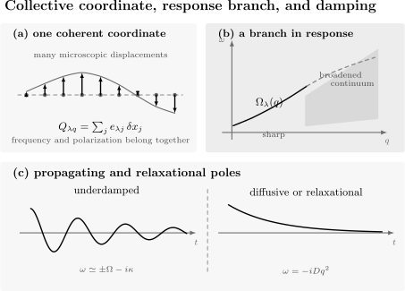
Three views of a collective mode. A mode coordinate combines many microscopic fluctuations with polarization $e_{\lambda j}$. In response space, an underdamped branch $\Omega_\lambda(q)$ can remain sharp outside a continuum and broaden after entering it. In time, collective dynamics may be oscillatory, with poles near $\pm\Omega-i\kappa$, or relaxational, with a pole such as $-iDq^2$.

Collective Modes in Exact Spectra

Lehmann representation

For a collective operator $O_{\mathbf q}$ at zero temperature,

$$\begin{aligned} S_O(\mathbf q,\omega) \propto{}& \sum_n \left| \langle n| O_{\mathbf q} |0\rangle \right|^2 \\ &\times \delta \left( \omega-\omega_{n0} \right). \end{aligned}$$

A collective mode appears when substantial operator weight organizes into a coherent branch or controlled pole.

The exact eigenstates remain the foundation. “Collective mode” is an interpretation of their energies, matrix elements, scaling, and dynamical organization.

Single-mode dominance

If one state exhausts most of the relevant spectral weight,

$$S_O(\mathbf q,\omega) \simeq Z_O(\mathbf q) \delta \left( \omega-\Omega(\mathbf q) \right)$$

in an ideal stable limit.

The single-mode approximation can be powerful, but its quality must be checked against:

• omitted weight;
• multiparticle continua;
• sum rules;
• finite-size level spacing;
• operator dependence.

Feynman-type variational state

A density collective trial state has the schematic form

$$|\mathbf q\rangle \propto \rho_{\mathbf q}|0\rangle.$$

Its variational energy connects static structure to an excitation estimate. This does not prove exact single-mode saturation.

Sum Rules owns the exact moment derivation and Feynman bound.

Continuum without a mode

A collective operator can couple mainly to a continuum:

$$S_O = S_{\mathrm{cont}}$$

with no isolated pole. The operator is collective, but the spectrum need not contain a sharp collective mode.

This distinction matters near quantum critical points, in one-dimensional fractionalized systems, and in strongly damped metals.

Collective Modes and Particle–Hole Continua

Coherent superposition

In a fermionic reference state, a density-like collective excitation can have the leading form

$$\begin{aligned} |\lambda,\mathbf q\rangle \sim{}& \sum_{\mathbf k} \phi_{\lambda\mathbf q}(\mathbf k) \\ &\times c_{\mathbf k+\mathbf q}^\dagger c_{\mathbf k} |\Psi_0\rangle + \cdots. \end{aligned}$$

The coherent superposition across many $\mathbf k$ values distinguishes a collective eigenvector from one selected particle–hole configuration.

Continuum kinematics

The set of individual particle–hole energies

$$\omega = \frac{ \epsilon_{\mathbf k+\mathbf q} - \epsilon_{\mathbf k} }{ \hbar }$$

fills a continuum as $\mathbf k$ varies.

Interactions can pull or organize a pole outside that continuum. Inside it, resonant decay often broadens the mode.

No universal percentage

There is no universal threshold such as “more than half the particles participate.” A mode can be collective because:

• its eigenvector is a coherent superposition;
• its frequency is set by a self-consistent field;
• its residue scales coherently;
• it is governed by a hydrodynamic variable;
• it is protected by symmetry or conservation.

The relevant criterion depends on the problem.

Methods for Finding Collective Modes

Exact response

In principle, collective modes are read from exact retarded correlators or structure factors. In practice, exact spectra are available only in special models or finite numerical systems.

Time-dependent mean field

Linearizing a time-dependent mean-field equation around a stationary saddle produces small-oscillation modes. Examples include:

• time-dependent Hartree or Hartree–Fock;
• Gross–Pitaevskii and Bogoliubov–de Gennes equations;
• time-dependent density-functional approximations;
• linearized Landau kinetic theory.

The mode solution is only as controlled as the background and closure.

Random phase approximation

RPA solves a self-consistent response problem. In a scalar density channel,

$$\chi_{\mathrm{RPA}} = \frac{ \chi_0 }{ 1-V\chi_0 }.$$

A collective pole can satisfy

$$1 - V(\mathbf q) \chi_0(\mathbf q,\omega) = 0.$$

The numerator and imaginary part of $\chi_0$ still determine visibility and damping. Random Phase Approximation owns signs, screening, Lindhard functions, sum rules, and validity.

Effective action

For fields $\Phi_a$, expand an effective action about a saddle:

$$S_{\mathrm{eff}} = S_0 + \frac12 \sum_{ab} \delta\Phi_a \mathcal K_{ab} \delta\Phi_b + \cdots.$$

After the correct real-time continuation, zeros of $\det\mathcal K^{\mathrm R}$ give collective poles.

An imaginary-time Hessian alone does not determine retarded damping without analytic continuation.

Hydrodynamics

At long wavelength and low frequency, conservation laws and constitutive relations can determine pole structure without solving microscopic dynamics.

Hydrodynamics predicts the functional form of slow modes. Microscopic theory supplies thermodynamic derivatives and transport coefficients.

Equation-of-motion and moment methods

Commutators generate exact spectral moments:

$$\langle [O^\dagger,[H,O]] \rangle.$$

Moment constraints can bound or estimate collective energies, but a finite number of moments cannot by itself distinguish a narrow pole from every possible continuum.

Numerical spectra

Exact diagonalization, tensor networks, quantum Monte Carlo with analytic continuation, and real-time simulation can reveal candidate modes.

Necessary controls include:

• system-size scaling;
• frequency broadening or time-window scaling;
• momentum resolution;
• operator normalization;
• boundary conditions;
• analytic-continuation uncertainty;
• sum-rule closure;
• comparison across several channels.

Observing Collective Modes

Scattering probes

Neutron, x-ray, electron-energy-loss, and Bragg scattering access momentum- and frequency-resolved correlations.

The measured intensity is schematically

$$\begin{aligned} I(\mathbf q,\omega) \sim{}& \mathbf f^\dagger \left[ -\operatorname{Im} \chi^{\mathrm R} (\mathbf q,\omega) \right] \mathbf f \\ &\ast \mathcal R(\mathbf q,\omega) + \text{background}, \end{aligned}$$

with probe vertices $\mathbf f$ and resolution kernel $\mathcal R$.

Optical and Raman probes

Photons carry little crystal momentum in ordinary optical geometries, so these probes emphasize near-zone-center modes and symmetry-selected channels.

A mode can be Raman active, infrared active, both, or neither depending on symmetry and effective charge.

Pump–probe dynamics

A short perturbation can launch coherent oscillations:

$$\delta O(t) \sim A e^{-\kappa t} \cos \left( \Omega t+\varphi \right).$$

The observed frequency and damping can identify a mode, but nonlinear driving, heating, inhomogeneity, and multiple beating frequencies must be controlled.

Transport and thermodynamics

Collective modes affect:

• thermal conductivity;
• sound attenuation;
• optical conductivity;
• heat capacity;
• drag and viscosity;
• critical relaxation.

These integrated observables constrain a mode description but usually do not determine its complete dispersion and polarization.

A convergence standard

A strong experimental or numerical identification combines:

1. a reproducible branch or pole;
2. symmetry-consistent polarization;
3. source and detector selection rules;
4. controlled intrinsic width;
5. spectral-weight and sum-rule accounting;
6. finite-size or resolution scaling;
7. agreement with an independently measured thermodynamic or transport parameter;
8. a method whose validity covers the claimed regime.

One peak at one momentum is not yet a collective-mode theory.

A Practical Mode Checklist

Name the background

Specify the equilibrium, ordered, metastable, or driven state around which fluctuations are defined.

Name the coordinate

State what oscillates:

$$\delta n, \quad \delta\mathbf M, \quad \mathbf u, \quad \theta, \quad h, \quad \ldots$$

State the dynamical regime

Declare:

• hydrodynamic or collisionless;
• conservative or dissipative;
• isolated or open;
• linear or nonlinear;
• finite or thermodynamic.

Derive the kernel

Write the linearized equations or inverse response matrix. Do not infer a mode solely from terminology.

Solve for frequency and polarization

Report both

$$\omega_\lambda(\mathbf q)$$

and

$$\mathbf e_\lambda(\mathbf q).$$

Project onto the probe

Check whether the chosen source and detector couple to the eigenvector.

Locate continua

Identify decay thresholds and overlapping branches.

Quantify damping

Compare

$$\lvert\operatorname{Im}\omega_\lambda\rvert$$

with the relevant real frequency, branch separation, and experimental resolution.

Check scaling

Vary:

• size;
• momentum;
• broadening;
• boundary conditions;
• temperature;
• control parameters.

State the cutoff

Give the wavelength, frequency, amplitude, and occupation range over which the mode description is intended.

Common Mistakes

Calling every many-body excitation collective

All exact excitations belong to a many-body Hilbert space. Collectivity requires a coherent coordinate, eigenvector, self-consistent field, hydrodynamic variable, or comparable organizing structure.

Requiring macroscopic occupation

A single quantum of an extended normal mode is collective. Macroscopic occupation creates a classical wave but is not the definition.

Assuming collective means gapless

Plasmons, optical phonons, amplitude modes, and relative-phase modes can be gapped.

Assuming collective means sharp

Diffusion and overdamped order-parameter relaxation are collective. Sharpness determines quasiparticle usefulness, not collectivity alone.

Calling every pole a collective mode

A finite-system single-particle transition is a pole. Collective identification also requires operator structure, polarization, scaling, or a coherent branch.

Ignoring the numerator

A zero of a response denominator can be dark in the chosen channel or canceled by a vanishing numerator. Compute the residue.

Using a scalar response for coupled variables

Amplitude, phase, density, current, sublattice, and component channels can mix. Diagonalizing one diagonal entry can miss the true eigenmodes.

Sorting branches only by energy

Near an avoided crossing, mode character transfers between energy-ordered branches. Track eigenvectors and spectral weight.

Confusing a continuum edge with a mode

A threshold can produce a strong peak or cusp without an isolated pole. Test line shape, analytic structure, and resolution dependence.

Calling every amplitude feature a Higgs mode

Establish an amplitude-like eigenvector, symmetry channel, pole or controlled resonance, and separation from pair-breaking or multiparticle continua.

Ignoring long-range Coulomb coupling

A neutral phase mode and a charged longitudinal mode can have qualitatively different long-wavelength spectra.

Mixing first sound and zero sound

The distinction depends on $\omega\tau_{\mathrm{coll}}$. A formula from one regime should not be applied in the other without a crossover treatment.

Treating RPA as exact

RPA can reveal real collective physics while remaining an approximation with missing exchange, vertex, local-field, or strong-correlation effects.

Treating participation ratio as invariant

Participation depends on basis, metric, and normalization. Use it with physical operator and scaling information.

Exercises

Exercise 1: In-phase and out-of-phase oscillations

For the coupled-oscillator Lagrangian

$$\begin{aligned} L ={}& \frac{m}{2} \left( \dot x_1^2+\dot x_2^2 \right) \\ &- \frac{k_0}{2} \left( x_1^2+x_2^2 \right) \\ &- \frac{k_c}{2} \left( x_1-x_2 \right)^2, \end{aligned}$$

derive the normal coordinates and frequencies. Which mode couples to a uniform force $F(x_1+x_2)$?

Solution

Use

$$Q_\pm = \frac{x_1\pm x_2}{\sqrt2}.$$

The inverse transformation is

$$x_1 = \frac{Q_++Q_-}{\sqrt2}, \qquad x_2 = \frac{Q_+-Q_-}{\sqrt2}.$$

Then

$$x_1^2+x_2^2 = Q_+^2+Q_-^2$$

and

$$\left( x_1-x_2 \right)^2 = 2Q_-^2.$$

Therefore

$$\begin{aligned} L ={}& \frac{m}{2} \left( \dot Q_+^2+\dot Q_-^2 \right) \\ &- \frac{k_0}{2}Q_+^2 \\ &- \frac{k_0+2k_c}{2}Q_-^2. \end{aligned}$$

The frequencies are

$$\omega_+ = \sqrt{\frac{k_0}{m}}, \qquad \omega_- = \sqrt{ \frac{k_0+2k_c}{m} }.$$

The uniform force couples through

$$F(x_1+x_2) = \sqrt2FQ_+.$$

It excites only the in-phase mode. The out-of-phase mode exists but is dark to a perfectly uniform symmetric source.

Exercise 2: A denominator zero can be dark

Suppose the response in the $Q_\pm$ basis is

$$\chi_\pm^{\mathrm R}(\omega) = \frac{1}{ \Omega_\pm^2 - (\omega+i0^+)^2 }.$$

A source and detector both couple only to $O=X_1+X_2$. Show which pole appears in $\chi_{OO}^{\mathrm R}$.

Solution

Since

$$O = X_1+X_2 = \sqrt2Q_+,$$

the source and detector have no projection onto $Q_-$. Therefore

$$\chi_{OO}^{\mathrm R} = 2\chi_+^{\mathrm R}.$$

The poles at $\omega=\pm\Omega_+$ appear, while the poles at $\pm\Omega_-$ have zero residue in this channel.

The antisymmetric mode is not absent from the system. It requires an antisymmetric source or detector such as $X_1-X_2$.

Exercise 3: Underdamped or overdamped?

For

$$\ddot Q + 2\kappa\dot Q + \Omega_0^2Q = 0,$$

classify the motion for:

1. $\kappa=\Omega_0/10$;
2. $\kappa=\Omega_0$;
3. $\kappa=2\Omega_0$.

Find the poles in each case.

Solution

The poles are

$$\omega_\pm = -i\kappa \pm \sqrt{ \Omega_0^2-\kappa^2 }.$$

For $\kappa=\Omega_0/10$,

$$\omega_\pm = -\frac{i\Omega_0}{10} \pm \frac{\sqrt{99}}{10} \Omega_0.$$

The poles have nonzero real parts and the mode is underdamped.

For $\kappa=\Omega_0$,

$$\omega_+ = \omega_- = -i\Omega_0.$$

This is critical damping in the elementary model.

For $\kappa=2\Omega_0$,

$$\omega_\pm = -2i\Omega_0 \pm i\sqrt3\,\Omega_0.$$

Both poles lie on the negative imaginary axis:

$$\omega_\pm = -i \left( 2\mp\sqrt3 \right) \Omega_0.$$

The response is overdamped and relaxes as a sum of two exponentials.

Exercise 4: Diffusion from conservation

Starting from

$$\partial_t n + \nabla\cdot\mathbf j = 0$$

and

$$\mathbf j = -D\nabla n,$$

derive the dispersion and explain why the mode is collective but not a ballistic quasiparticle.

Solution

Substitution gives

$$\partial_t n = D\nabla^2n.$$

For

$$\delta n = \delta n_0 e^{i(\mathbf q\cdot\mathbf r-\omega t)},$$

one finds

$$-i\omega = -Dq^2,$$

so

$$\omega = -iDq^2.$$

The mode is collective because it describes coherent long-wavelength relaxation of the conserved density field. Its pole has no real oscillation frequency, so there is no ballistic wave packet with a group velocity. Particle-like quasiparticle language is therefore generally inappropriate.

Exercise 5: Derive neutral sound

Use

$$\partial_t\delta n + n_0\nabla\cdot\mathbf v = 0$$

and

$$mn_0\partial_t\mathbf v = -\nabla \left[ \left( \frac{\partial P}{\partial n} \right)_{\!s} \delta n \right]$$

to derive the sound speed.

Solution

Differentiate continuity with respect to time:

$$\partial_t^2\delta n + n_0\nabla\cdot \partial_t\mathbf v = 0.$$

From the Euler equation,

$$\partial_t\mathbf v = - \frac{1}{mn_0} \left( \frac{\partial P}{\partial n} \right)_{\!s} \nabla\delta n.$$

Substitution gives

$$\partial_t^2\delta n - \frac{1}{m} \left( \frac{\partial P}{\partial n} \right)_{\!s} \nabla^2\delta n = 0.$$

Thus

$$\partial_t^2\delta n = c_s^2\nabla^2\delta n$$

with

$$c_s^2 = \frac{1}{m} \left( \frac{\partial P}{\partial n} \right)_{\!s}.$$

Plane waves have

$$\omega_\pm = \pm c_sq.$$

Exercise 6: Participation is basis dependent

In a site basis, let

$$e_j = \frac{1}{\sqrt N}$$

for every $j$. Compute the participation ratio. Then transform to a basis whose first vector is exactly $\mathbf e$. What participation ratio does the same mode have there?

Solution

In the site basis,

$$\sum_j \lvert e_j\rvert^4 = N \left( \frac{1}{N^2} \right) = \frac1N.$$

Therefore

$$P = \frac{1}{1/N} = N.$$

Now choose an orthonormal basis with first basis vector $\mathbf u_1=\mathbf e$. The same mode has components

$$\left( 1,0,\ldots,0 \right).$$

In that basis,

$$P = 1.$$

The physics did not change. The example proves that participation ratio is basis dependent and must be interpreted in a physically motivated local or component basis.

Exercise 7: Avoided crossing and character exchange

For

$$\mathcal K = \begin{pmatrix} \omega-\omega_1 & -g \\ -g & \omega-\omega_2 \end{pmatrix},$$

derive the two frequencies. At $\omega_1=\omega_2=\omega_0$, find normalized eigenvectors.

Solution

The determinant condition is

$$\left( \omega-\omega_1 \right) \left( \omega-\omega_2 \right) - g^2 = 0.$$

Solving the quadratic gives

$$\begin{aligned} \omega_\pm ={}& \frac{\omega_1+\omega_2}{2} \\ &\pm \sqrt{ \left( \frac{\omega_1-\omega_2}{2} \right)^2 +g^2 }. \end{aligned}$$

At degeneracy,

$$\omega_\pm = \omega_0 \pm \lvert g\rvert.$$

For $g>0$, the normalized eigenvectors can be chosen as

$$\mathbf e_+ = \frac{1}{\sqrt2} \begin{pmatrix} 1\\-1 \end{pmatrix}, \qquad \mathbf e_- = \frac{1}{\sqrt2} \begin{pmatrix} 1\\1 \end{pmatrix}.$$

The splitting is $2g$. Away from the crossing, the eigenvectors rotate continuously between the original coordinate characters.

Exercise 8: Audit a claimed collective mode

A numerical calculation on one finite lattice shows a broad maximum in a density structure factor at one momentum. The plot uses artificial Lorentzian broadening $\eta=0.15J$. The fitted FWHM is $0.18J$, and the feature is labeled a long-lived collective mode.

List the missing checks.

Solution

The fitted width is comparable to the artificial broadening, so it does not establish an intrinsic lifetime. A broad maximum at one momentum can be:

• one broadened discrete line;
• several unresolved levels;
• a continuum threshold;
• a density-of-states enhancement;
• the finite-size precursor of a resonance;
• a genuine collective branch.

A responsible analysis should:

1. repeat the calculation for several $\eta$ values;
2. inspect raw finite-size energies and matrix elements;
3. scale system size and boundary conditions;
4. trace the feature across momentum;
5. compare with the particle–hole or multiparticle continuum;
6. identify its polarization or dominant operator eigenchannel;
7. check spectral moments and total weight;
8. compare density response with another appropriate channel;
9. test a linearized effective or hydrodynamic prediction;
10. show that an intrinsic width remains after resolution and finite-size effects are controlled.

Until then, “candidate density-response feature” is more accurate than “long-lived collective mode.”

Key Takeaways

• A collective mode is a coherent dynamical pattern or response eigenchannel built from many microscopic degrees of freedom.
• Collectivity is defined relative to variables, background, scale, approximation, and probe.
• A mode can be identified as a collective coordinate, a homogeneous solution of linearized dynamics, or a pole of a response matrix.
• Frequency, polarization, residue, damping, and regime are independent pieces of mode data.
• Normal mode, collective mode, quasiparticle, resonance, coherent state, and exact eigenstate are related but distinct concepts.
• One quantum can be collective; macroscopic occupation is not required.
• Conservation laws produce hydrodynamic modes such as diffusion and sound.
• Broken symmetries can enforce Goldstone modes, but many collective modes are gapped or unrelated to symmetry breaking.
• Long-range Coulomb feedback can convert a neutral acoustic phase or density mode into a gapped plasma oscillation.
• Coupled channels hybridize, avoid crossings, exchange character, and can be bright or dark depending on the probe.
• A continuum can damp or dissolve a mode; a strong threshold feature is not automatically an isolated pole.
• Participation ratio is useful but basis dependent.
• A convincing identification combines dispersion, polarization, residue, intrinsic width, sum rules, scaling, and a controlled dynamical model.

Further Reading

• For particle-like criteria and the overlap between collective modes and quasiparticles, see Quasiparticles Overview.
• For exact response conventions, see Retarded and Advanced Response and Susceptibilities.
• For measured scattering spectra, see Structure Factors.
• For peak, continuum, residue, and linewidth conventions, see Spectral Functions.
• For dielectric collective poles, see Random Phase Approximation.
• For symmetry-enforced modes, see Goldstone Modes in Many-Body Systems.
• For force constants, real-crystal phonon dispersions, vibrational thermodynamics, and probe interpretation, see Phonons.
• For selecting conserved slow fields and organizing their constitutive, fluctuation, and effective-theory expansions, see Hydrodynamics and Effective Theory Preview.
• For a materials-facing sequence, see the Condensed Matter Roadmap.

References

• D. Bohm and D. Pines, “A Collective Description of Electron Interactions: III. Coulomb Interactions in a Degenerate Electron Gas”, Physical Review 92, 609–625, 1953.
• L. D. Landau, “Oscillations in a Fermi Liquid”, Soviet Physics JETP 5, 101–108, 1957; received in 1956.
• R. P. Feynman, “Atomic Theory of the Two-Fluid Model of Liquid Helium”, Physical Review 94, 262–277, 1954.
• R. Kubo, “Statistical-Mechanical Theory of Irreversible Processes. I”, Journal of the Physical Society of Japan 12, 570–586, 1957.
• L. Van Hove, “Correlations in Space and Time and Born Approximation Scattering in Systems of Interacting Particles”, Physical Review 95, 249–262, 1954.
• P. W. Anderson, “Random-Phase Approximation in the Theory of Superconductivity”, Physical Review 112, 1900–1916, 1958.
• L. P. Kadanoff and P. C. Martin, “Hydrodynamic Equations and Correlation Functions”, Annals of Physics 24, 419–469, 1963.
• W. Kohn, “Cyclotron Resonance and de Haas–van Alphen Oscillations of an Interacting Electron Gas”, Physical Review 123, 1242–1244, 1961.
• P. B. Littlewood and C. M. Varma, “Amplitude Collective Modes and Coupling to Charge-Density Waves in Superconductors”, Physical Review B 26, 4883–4893, 1982.
• P. C. Hohenberg and B. I. Halperin, “Theory of Dynamic Critical Phenomena”, Reviews of Modern Physics 49, 435–479, 1977.
• A. L. Fetter and J. D. Walecka, Quantum Theory of Many-Particle Systems, Dover, 2003.
• D. Pines and P. Nozières, The Theory of Quantum Liquids, Volume I: Normal Fermi Liquids, CRC Press, 2018 reissue.
• G. D. Mahan, Many-Particle Physics, 3rd ed., Springer, 2000.
• A. Griffin, Excitations in a Bose-Condensed Liquid, Cambridge University Press, 1993.
• L. P. Pitaevskii and S. Stringari, Bose–Einstein Condensation and Superfluidity, Oxford University Press, 2016.
• D. Forster, Hydrodynamic Fluctuations, Broken Symmetry, and Correlation Functions, CRC Press reissue, 2018.
• P. Coleman, Introduction to Many-Body Physics, Cambridge University Press, 2015.
• A. Altland and B. Simons, Condensed Matter Field Theory, 2nd ed., Cambridge University Press, 2010.