Heisenberg Model

The Heisenberg model describes fixed-length quantum spins coupled by rotationally invariant exchange. On a nearest-neighbor lattice its canonical Hamiltonian is

$$H = J \sum_{\langle i,j\rangle} \mathbf s_i\cdot\mathbf s_j,$$

where the dimensionless spin operators obey $\mathbf s_i^2=s(s+1)$. With this sign convention, $J\gt0$ is antiferromagnetic and $J\lt0$ is ferromagnetic.

The formula is compact, but its behavior depends decisively on spin $s$, dimension, lattice geometry, boundary conditions, temperature, and the sign and range of exchange. It includes exact dimers and ferromagnetic one-magnon states, the Bethe-ansatz-solvable spin-$1/2$ chain, semiclassical ordered magnets, frustrated lattices, and the integer-spin Haldane regime. It is therefore both a model of localized quantum magnetism and a laboratory for symmetry, entanglement, collective modes, criticality, and emergence.

Canonical Scope

The Heisenberg Chain dossier is the convention-complete lookup record for the uniform spin-$1/2$ chain, its exact fingerprints, and its numerical contract. This teaching article owns the broader derivations and physical interpretation across spin, graph, dimension, and approximation regime.

This page is the canonical home for the isotropic Heisenberg model: its Hilbert space, exchange convention, symmetries, elementary exact limits, one-dimensional benchmarks, spin-wave preview, observables, and solution status. The Spin-$1/2$ Chain dossier owns the umbrella XYZ-family record, cross-model normalization, generic sector audit, and shared matrix checks. Lattice Models Overview supplies the graph, locality, support, interaction, and effective-model language.

The underlying spin algebra and addition of angular momentum are developed in the symmetry volume. Goldstone Modes in Many-Body Systems owns the symmetry counting that distinguishes the ferromagnet’s one type-B magnon from the collinear antiferromagnet’s two type-A modes. The controlled strong-coupling projection from the half-filled repulsive Hubbard model owns the lattice derivation of $J=4t^2/U$. For a material record, Magnetism and Spin Systems routes the declared moment, coupling, state, observable, and evidence to the appropriate mechanism, phase, or excitation owner; full computational algorithms remain in their dedicated volumes.

The word Heisenberg also names the Heisenberg picture and Heisenberg equation of motion. Those are general formulations of quantum dynamics, not this particular lattice Hamiltonian.

Degrees of Freedom and Units

Choose a graph $G=(V,E)$ with $L=|V|$ sites. Each site carries one irreducible spin-$s$ degree of freedom,

$$\mathcal H_i \simeq \mathbb C^{2s+1}.$$

The many-spin Hilbert space is

$$\mathcal H = \bigotimes_{i=1}^{L} \mathcal H_i, \qquad \dim\mathcal H = (2s+1)^L.$$

Dimensionless spin operators satisfy

$$\begin{aligned} [s_i^\alpha,s_j^\beta] &= i\delta_{ij} \epsilon_{\alpha\beta\gamma} s_i^\gamma, \\ \mathbf s_i^2 &= s(s+1), \end{aligned}$$

with $\alpha,\beta,\gamma\in\{x,y,z\}$. Operators on different sites commute.

Physical angular momentum is

$$\mathbf S_i = \hbar\mathbf s_i.$$

Accordingly, the same exchange term can be written in either of two equivalent conventions:

$$J\mathbf s_i\cdot\mathbf s_j = \frac{J}{\hbar^2} \mathbf S_i\cdot\mathbf S_j.$$

Here $J$ has units of energy. A formula written directly as $J\mathbf S_i\cdot\mathbf S_j$ instead assigns different units to its symbol $J$. Numerical comparisons require checking this convention first.

For spin $1/2$,

$$\mathbf s_i = \frac{1}{2}\boldsymbol\sigma_i, \qquad \mathbf S_i = \frac{\hbar}{2}\boldsymbol\sigma_i.$$

Hamiltonian on a Graph

The isotropic exchange Hamiltonian on a general graph is

$$H_{ \mathrm{ex} } = \sum_{(i,j)\in E} J_{ij} \mathbf s_i\cdot\mathbf s_j.$$

Each unordered bond should appear once. For a uniform nearest-neighbor model,

$$H = J \sum_{\langle i,j\rangle} \mathbf s_i\cdot\mathbf s_j.$$

A field measured in energy units adds

$$H_h = -\sum_i \mathbf h_i\cdot\mathbf s_i.$$

If the physical magnetic field is $\mathbf B_i$ and the magnetic moment convention is $\boldsymbol\mu_i=g\mu_{mathrm B}\mathbf s_i$, then $\mathbf h_i=g\mu_{mathrm B}\mathbf B_i$. The electron magnetic moment may introduce an additional sign depending on whether the spin or magnetic-moment direction is being described.

Common extensions include anisotropic exchange,

$$H_{XYZ} = \sum_{\langle i,j\rangle} \left( J_xs_i^xs_j^x + J_ys_i^ys_j^y + J_zs_i^zs_j^z \right),$$

single-ion anisotropy $D\sum_i(s_i^z)^2$ for $s\ge1$, antisymmetric Dzyaloshinskii–Moriya exchange, longer-range couplings, and multi-spin terms. These are related models. They can change the symmetry, spectrum, ordering, and even the phase classification, so results for the isotropic model should not be transferred to them silently.

What the Sign of Exchange Means

For one bond, define its total spin

$$\mathbf s_{ij} = \mathbf s_i+\mathbf s_j.$$

The identity

$$\mathbf s_i\cdot\mathbf s_j = \frac{1}{2} \left( \mathbf s_{ij}^2 - \mathbf s_i^2 - \mathbf s_j^2 \right)$$

diagonalizes the exchange interaction in sectors of bond spin $\ell=0,1,\ldots,2s$. The corresponding bond energy is

$$E_\ell = \frac{J}{2} \left[ \ell(\ell+1) - 2s(s+1) \right].$$

Thus:

• $J\gt0$ favors the smallest available bond spin and is called antiferromagnetic;
• $J\lt0$ favors the largest bond spin and is called ferromagnetic.

These names describe the energetic tendency of each exchange bond. They do not by themselves prove long-range order. Quantum fluctuations, frustration, dimensionality, and temperature determine whether an ordered phase actually forms.

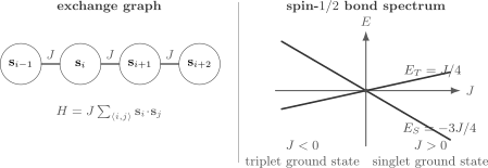
An isotropic bond couples fixed-length spins through $J\mathbf s_i\cdot\mathbf s_j$. For two spin-$1/2$ sites, $J\lt0$ places the triplet below the singlet, whereas $J\gt0$ places the singlet below the triplet. The crossing at $J=0$ makes the sign convention explicit.

Exact Spin-One-Half Dimer

The two-site spin-$1/2$ model is the basic exchange benchmark:

$$H_{ 2 } = J\mathbf s_1\cdot\mathbf s_2.$$

The singlet is

$$\lvert S\rangle = \frac{ \lvert\uparrow\downarrow\rangle - \lvert\downarrow\uparrow\rangle }{\sqrt2},$$

and the triplet is

$$\begin{aligned} \lvert T_+\rangle &= \lvert\uparrow\uparrow\rangle, \\ \lvert T_0\rangle &= \frac{ \lvert\uparrow\downarrow\rangle + \lvert\downarrow\uparrow\rangle }{\sqrt2}, \\ \lvert T_-\rangle &= \lvert\downarrow\downarrow\rangle. \end{aligned}$$

Their energies are

$$E_S = -\frac{3J}{4}, \qquad E_T = \frac{J}{4}.$$

The singlet–triplet gap, defined as $E_T-E_S$, is exactly $J$. Antiferromagnetic exchange selects the entangled singlet; ferromagnetic exchange selects the three-dimensional triplet multiplet.

The exchange operator also has useful projector forms:

$$\begin{aligned} P_S &= \frac{1}{4} - \mathbf s_1\cdot\mathbf s_2, \\ P_T &= \frac{3}{4} + \mathbf s_1\cdot\mathbf s_2. \end{aligned}$$

For spin $1/2$, the swap operator is

$$P_{12} = 2\mathbf s_1\cdot\mathbf s_2 + \frac{1}{2}.$$

This identity links exchange, permutation symmetry, and singlet–triplet splitting. It is special to two spin-$1/2$ degrees of freedom in this simple form.

Thermal dimer

At inverse temperature $\beta$, the dimer partition function is

$$Z_2 = e^{3\beta J/4} + 3e^{-\beta J/4}.$$

The factor of three is the triplet degeneracy. The exact exchange correlation is

$$\left\langle \mathbf s_1\cdot\mathbf s_2 \right\rangle_\beta = -\frac{3}{4} \frac{ e^{\beta J}-1 }{ e^{\beta J}+3 }.$$

It approaches zero at high temperature. At low temperature it approaches $-3/4$ for $J\gt0$ and $1/4$ for $J\lt0$. This exactly solvable system is a useful check on thermal-state normalization, degeneracy factors, energy derivatives, and sign conventions.

Global Spin-Rotation Symmetry

Define total spin

$$\mathbf s_{ \mathrm{tot} } = \sum_i\mathbf s_i.$$

Every isotropic bond is a scalar under simultaneous rotations of all spins. Therefore

$$[H,s_{ \mathrm{tot} }^\alpha] = 0, \qquad \alpha\in\{x,y,z\},$$

and

$$[H,\mathbf s_{ \mathrm{tot} }^2] = 0.$$

The model has global $SU(2)$ spin-rotation symmetry. Its energy eigenstates can be organized into total-spin multiplets labeled by $S_{mathrm{tot}}$ and $m$. Within an exact multiplet the energy is independent of $m$.

This global symmetry does not mean that each local spin is conserved. In general,

$$[H,\mathbf s_i] \ne 0,$$

because exchange transfers angular momentum between sites while preserving the total.

Additional symmetries depend on the graph and couplings:

• a uniform chain or Bravais lattice may have translations and point-group symmetries;
• real isotropic exchange without a field is invariant under time reversal;
• spatial inversion may exchange sites or bonds;
• a uniform field leaves rotations about the field axis and conserves the corresponding total magnetization;
• XXZ anisotropy usually retains a $U(1)$ subgroup, while generic XYZ anisotropy retains less.

Symmetry sectors reduce numerical cost and provide strict checks on spectra and matrix elements.

Chains and Boundary Conditions

For a one-dimensional chain of $L$ sites,

$$H_{ \mathrm{chain} } = J \sum_i \mathbf s_i\cdot\mathbf s_{i+1}.$$

The range of the sum must be stated:

$$\begin{array}{ll} i=1,\ldots,L-1 &\text{open boundary conditions}, \\ i=1,\ldots,L, \quad \mathbf s_{L+1}=\mathbf s_1 &\text{periodic boundary conditions}. \end{array}$$

The open chain has $L-1$ bonds; the periodic chain has $L$ bonds. For an antiferromagnetic periodic chain, odd $L$ prevents a perfectly alternating pattern and introduces geometric frustration. These finite-size details can alter degeneracies, momentum quantum numbers, edge states, and gaps.

Ferromagnetic Ground States

Let $J\lt0$ on every bond of a connected nearest-neighbor graph. The fully polarized state

$$\lvert F\rangle = \lvert s,s,\ldots,s\rangle$$

has maximal spin on every bond and is an exact ground state. Global rotations generate the maximal-total-spin multiplet

$$S_{ \mathrm{tot} } = Ls,$$

with $2Ls+1$ states. On a periodic uniform chain its energy is

$$E_F = JLs^2.$$

For open boundaries, replace $L$ by $L-1$ in the bond count.

The polarized product state is exact because every ferromagnetic bond can minimize its energy simultaneously. This is very different from an antiferromagnet, where minimizing one bond through a singlet generally conflicts with sharing each spin among several bonds.

Exact one-magnon dispersion

On a periodic chain, create one localized spin deviation with

$$\lvert j\rangle = \frac{1}{\sqrt{2s}} s_j^- \lvert F\rangle.$$

Within the one-deviation subspace,

$$\left( H-E_F \right) \lvert j\rangle = Js \left( \lvert j-1\rangle + \lvert j+1\rangle - 2\lvert j\rangle \right).$$

Momentum states

$$\lvert k\rangle = \frac{1}{\sqrt L} \sum_j e^{ikaj} \lvert j\rangle$$

are therefore exact eigenstates with excitation energy

$$\varepsilon(k) = 2\lvert J\rvert s \left[ 1-\cos(ka) \right].$$

Near $k=0$,

$$\varepsilon(k) \simeq \lvert J\rvert s (ka)^2.$$

The $k=0$ state is proportional to $s_{mathrm{tot}}^-\lvert F\rangle$ and lies in the same ground multiplet. The quadratic long-wavelength dispersion is characteristic of an isotropic ferromagnet. On a finite periodic chain, the smallest nonzero momentum is $2\pi/(La)$, so the first dispersing magnon energy scales as $L^{-2}$.

Why the Antiferromagnet Is More Quantum

Write one bond as

$$\mathbf s_i\cdot\mathbf s_j = s_i^zs_j^z + \frac{1}{2} \left( s_i^+s_j^- + s_i^-s_j^+ \right).$$

On a bipartite lattice, the classical Néel product state alternates the largest positive and negative $s^z$ values. Its exchange expectation is

$$\left\langle \mathbf s_i\cdot\mathbf s_j \right\rangle_{ \mathrm{N\acute eel} } = -s^2$$

on each antiparallel bond. It is generally not an eigenstate, because the transverse terms exchange neighboring spin projections.

For a dimer the exact antiferromagnetic bond energy is

$$-Js(s+1),$$

which is lower than the product-state expectation $-Js^2$. The additional lowering is a direct signature of quantum fluctuations and, for the spin-$1/2$ dimer, entanglement.

On an extended lattice, one spin cannot form an independent singlet with every neighbor. The ground state must compromise among overlapping bonds. This competition underlies resonating valence-bond descriptions, reduced ordered moments, fractionalized excitations in selected systems, and the difficulty of frustrated antiferromagnets.

Exact Spin-One-Half Antiferromagnetic Chain

For $s=1/2$, $J\gt0$, periodic boundaries, and nearest-neighbor exchange, the one-dimensional model is integrable by Bethe ansatz. In a sector with $M$ down spins, a coordinate ansatz has the schematic form

$$\psi(x_1,\ldots,x_M) = \sum_P A(P) \exp\!\left( i\sum_{a=1}^{M} k_{P_a}x_a \right),$$

for ordered positions $x_1\lt\cdots\lt x_M$. Two-body scattering relates the amplitudes $A(P)$, and periodicity quantizes the rapidities. The factorized scattering structure is special: generic perturbations destroy Bethe-ansatz integrability even though translation and spin symmetry may remain.

In the thermodynamic limit, the exact ground-state energy per site is

$$\frac{E_0}{L} = J \left( \frac{1}{4} - \ln2 \right) \simeq -0.443147J.$$

The ground state is a total-spin singlet for even $L$, not a Néel product state. It has strong antiferromagnetic correlations but no nonzero staggered magnetization in the translation-invariant one-dimensional ground state.

The low-energy spectrum is gapless. Its elementary fractional excitations are spinons carrying spin $1/2$. A local spin probe has integer spin overall and, with periodic boundaries, accesses multi-spinon continua rather than an isolated single-spinon pole. The exact lower edge of the two-spinon continuum is

$$\varepsilon_{ \mathrm L }(q) = \frac{\pi J}{2} \left\lvert \sin(qa) \right\rvert.$$

This result gives a linear low-energy scale near the gapless wavevectors. Calling every feature a magnon would miss the continuum and the fractional quantum numbers of the one-dimensional antiferromagnet.

The Bethe ansatz supplies far more than these benchmark formulas, but a complete derivation belongs in a dedicated integrability treatment. Here its role is to anchor approximations and finite-size calculations against exact results.

Integer and Half-Integer Chains

Haldane’s semiclassical mapping of the antiferromagnetic spin-$s$ chain leads to an $O(3)$ nonlinear sigma model with topological angle

$$\theta = 2\pi s.$$

The mapping distinguishes integer and half-integer spin:

• integer-spin nearest-neighbor chains are expected to have a nonzero bulk gap and short-range spin correlations;
• half-integer chains are constrained against a unique, symmetric, trivially gapped ground state and the uniform isotropic chain is gapless.

This statement is a low-energy classification, not the claim that every Hamiltonian with integer or half-integer onsite spin behaves identically. Dimerization, frustration, anisotropy, enlarged unit cells, long-range interactions, or symmetry breaking can change the outcome.

For the isotropic spin-1 chain, high-precision numerical work gives the Haldane gap

$$\Delta_{ \mathrm H } \simeq 0.4105J.$$

An open spin-1 chain also supports effective spin-$1/2$ edge degrees of freedom whose splitting becomes exponentially small with length. The symmetry-protected interpretation and full phase diagram belong with many-body phases and quantum matter; the key point here is that changing the onsite spin can qualitatively change the infrared physics even when the Hamiltonian has the same algebraic form.

Spin-Wave Theory Preview

Spin-wave theory expands around an ordered reference state by representing spin deviations as bosons. Magnons owns the general quantization, ferromagnet–antiferromagnet comparison, probe matrix elements, interactions, and validity tests. For a spin locally aligned along $+z$, the exact Holstein–Primakoff representation is

$$\begin{aligned} s_i^z &= s-a_i^\dagger a_i, \\ s_i^+ &= \sqrt{ 2s-a_i^\dagger a_i } \,a_i, \\ s_i^- &= a_i^\dagger \sqrt{ 2s-a_i^\dagger a_i }. \end{aligned}$$

Expanding the square roots assumes that the spin-deviation density is small compared with $2s$. Keeping quadratic terms gives linear spin-wave theory.

For the ferromagnetic chain, the one-boson result reproduces the exact one-magnon dispersion. Interactions between magnons enter at higher boson number and higher order in the expansion.

For a nearest-neighbor bipartite antiferromagnet, one first rotates the local axes on one sublattice. On a hypercubic lattice, linear spin-wave theory gives

$$\varepsilon_{\mathbf k} = zJs \sqrt{ 1-\gamma_{\mathbf k}^{,2} },$$

where $z$ is the coordination number and

$$\gamma_{\mathbf k} = \frac{1}{z} \sum_{\boldsymbol\delta} e^{i\mathbf k\cdot\boldsymbol\delta}$$

averages over nearest-neighbor vectors. The formula is most reliable for large $s$, low spin-wave density, and phases with stable long-range or strong semiclassical order.

In one dimension it predicts a gapless antiferromagnetic mode, but for the spin-$1/2$ chain it gives neither the exact velocity nor the correct spinon-continuum interpretation. Agreement on gaplessness does not make the quasiparticle content exact.

Dimensionality and Temperature

The Mermin–Wagner theorem places a precise limit on thermal ordering. For one- or two-dimensional isotropic Heisenberg models with finite-range exchange, continuous spin-rotation symmetry prevents ferromagnetic or antiferromagnetic long-range order at any nonzero temperature.

The conditions matter:

• the theorem concerns nonzero temperature, not automatically the ground state;
• it assumes the relevant continuous symmetry is unbroken by the Hamiltonian;
• sufficiently long-range interactions, anisotropy, or interlayer coupling can change the conclusion;
• it forbids the stated long-range order, not all correlations, crossovers, or topological phenomena.

For example, the two-dimensional square-lattice antiferromagnet can have Néel order at zero temperature while having only a large but finite correlation length at every $T\gt0$. A weak interlayer coupling or easy-axis anisotropy can then support a finite-temperature transition in a real quasi-two-dimensional material. Finite-Temperature Phase Transitions owns the general transition criteria and the assumptions behind such dimensionality statements; Universality owns how dimension, order-parameter symmetry, anisotropy, and interaction range classify any resulting critical point.

Finite systems never exhibit spontaneous symmetry breaking in exactly the same way as the infinite system. A finite-volume ground state can be a symmetry eigenstate while low-lying states, correlation functions, and order-of-limits behavior reveal the approach to an ordered thermodynamic phase. Spontaneous Symmetry Breaking develops the Anderson tower, oriented wave packets, and source-selected limit.

Frustration and Exchange Geometry

For nonuniform exchange,

$$H = \sum_{i<j} J_{ij} \mathbf s_i\cdot\mathbf s_j,$$

the signs and graph geometry determine whether preferred bond correlations can coexist.

An antiferromagnetic triangle is the simplest geometric example. No collinear assignment can make all three neighboring pairs antiparallel. Quantum mechanically, the three bonds share spins and cannot all be singlets. Frustration can enlarge ground-state degeneracy, suppress conventional order, favor noncollinear correlations, or stabilize highly entangled phases.

Competing exchanges can frustrate even a bipartite lattice. In the square-lattice $J_1$–$J_2$ model, antiferromagnetic nearest- and next-nearest-neighbor couplings prefer incompatible patterns. Disorder can add another source of competition.

Frustration is not synonymous with a spin liquid. A frustrated model may order, dimerize, freeze, remain critical, or realize a spin-liquid regime depending on parameters and dimension. Establishing the phase requires observables and scaling, not geometry alone.

Microscopic Origins and Model Boundaries

The Heisenberg model usually describes localized moments after charge and orbital excitations have been integrated out or otherwise frozen. Several microscopic mechanisms can generate exchange, including direct orbital exchange, superexchange through virtual charge fluctuations, and indirect exchange mediated by itinerant carriers.

For the single-band repulsive Hubbard model at half filling and $U\gg\lvert t\rvert$, controlled elimination of virtual doublon–hole states gives

$$H_{ \mathrm{eff} } = J_{ \mathrm H } \sum_{\langle i,j\rangle} \left( \mathbf s_i\cdot\mathbf s_j - \frac{1}{4} \right) + O\!\left( \frac{t^4}{U^3} \right),$$

with

$$J_{ \mathrm H } = \frac{4t^2}{U} \gt 0.$$

The constant can be dropped at fixed half filling. The derivation and its validity conditions are canonical in Effective Hamiltonians in Many-Body Systems.

The simple formula $4t^2/U$ is not a universal exchange law. Multiple orbitals, Hund coupling, ligand paths, spin–orbit coupling, charge-transfer energies, and higher-order virtual processes can change the magnitude, sign, range, and tensor structure of exchange.

The Heisenberg model also omits mobile charge. Away from half filling, projected hopping survives in the t–J model at first order and a spin-only Hamiltonian is generally insufficient. Likewise, strongly itinerant magnets may not admit a fixed local-spin description over the scales of interest.

The Kondo Model Preview retains both a localized spin and an itinerant conduction bath. Its central issue is screening by exchange, not a graph containing only fixed spins.

Core Observables

Magnetization

The total magnetization operator in spin units is

$$\mathbf M = \sum_i\mathbf s_i.$$

On a bipartite lattice, a staggered magnetization is

$$\mathbf M_{ \mathrm{st} } = \sum_i \eta_i\mathbf s_i,$$

where $\eta_i=+1$ on one sublattice and $-1$ on the other. A nonzero finite-system value of $\langle\mathbf M_{\mathrm{st}}\rangle$ requires a symmetry-breaking state or field; the rotationally invariant diagnostic is often $\langle\mathbf M_{\mathrm{st}}^2\rangle$ and its scaling.

Spin correlations

Equal-time correlations are

$$C^{\alpha\beta}_{ij} = \left\langle s_i^\alpha s_j^\beta \right\rangle.$$

In an $SU(2)$-invariant state,

$$\left\langle s_i^\alpha s_j^\beta \right\rangle = \frac{\delta_{\alpha\beta}}{3} \left\langle \mathbf s_i\cdot\mathbf s_j \right\rangle.$$

This relation is a useful symmetry check. It need not hold in a symmetry-broken state, in a field, or with anisotropic exchange.

Static structure factor

For positions $\mathbf r_i$, one common normalization is

$$S(\mathbf q) = \frac{1}{L} \sum_{i,j} e^{-i\mathbf q\cdot(\mathbf r_i-\mathbf r_j)} \left\langle \mathbf s_i\cdot\mathbf s_j \right\rangle.$$

A peak near $\mathbf q=0$ indicates ferromagnetic correlations. On a one-dimensional bipartite chain, antiferromagnetic correlations peak near $q=\pi/a$. Peak height and width must be scaled with system size before inferring long-range order; Long-Range Order gives the canonical extensive-versus-subextensive test.

Dynamic structure factor

A frequency-resolved convention is

$$\begin{aligned} S^{\alpha\beta}(\mathbf q,\omega) ={}& \frac{1}{2\pi L} \int_{-\infty}^{\infty} dt\,e^{i\omega t} \\ &\times \sum_{i,j} e^{-i\mathbf q\cdot(\mathbf r_i-\mathbf r_j)} \left\langle s_i^\alpha(t)s_j^\beta(0) \right\rangle. \end{aligned}$$

The normalization, Fourier sign, and thermal convention vary across fields. The dynamic structure factor distinguishes sharp magnons from continua and connects directly to scattering probes after including form factors and experimental units.

Structure Factors owns those general conventions, detailed-balance checks, and neutron polarization factors.

Susceptibility and gap

If a uniform field enters as $-hM^z$, the zero-field static susceptibility is

$$\chi = \beta \left[ \left\langle (M^z)^2 \right\rangle - \left\langle M^z \right\rangle^2 \right].$$

Divide by $L$ for susceptibility per site. Multiplication by $(g\mu_{mathrm B})^2$ converts to the response of the physical magnetic moment when $h=g\mu_{mathrm B}B$.

For a finite system, the spectral gap is

$$\Delta_L = E_1(L)-E_0(L).$$

The relevant symmetry and momentum sector must be stated. Whether $\Delta_L$ tends to zero or a positive constant as $L\to\infty$ distinguishes gapless and gapped bulk behavior, but edge states can require comparing several sector-resolved gaps.

Exact and Approximate Solution Status

The model’s simple definition does not imply generic solvability.

Exact structures include:

• arbitrary two-spin dimers by angular-momentum addition;
• fully polarized ferromagnetic ground states on broad classes of graphs;
• the one-magnon ferromagnetic sector;
• the spin-$1/2$ nearest-neighbor chain and selected anisotropic relatives by Bethe ansatz;
• small clusters by direct diagonalization.

Common controlled or systematically improvable approaches include:

• spin-wave and $1/s$ expansions in semiclassical ordered regimes;
• high- and low-temperature expansions;
• perturbation theory around dimers, Ising limits, or strong fields;
• matrix-product-state and density-matrix-renormalization methods in one dimension;
• quantum Monte Carlo for suitable unfrustrated models without a sign obstruction;
• exact diagonalization and Krylov methods for finite clusters;
• tensor-network, series, and linked-cluster methods in selected higher-dimensional settings.

No method is uniformly best. Frustration can create a Monte Carlo sign problem; two-dimensional entanglement growth limits tensor networks; spin-wave theory can fail without stable order; and exact diagonalization is exponentially size limited.

Finite-Size and Numerical Checks

A trustworthy calculation should record:

1. spin $s$, lattice, couplings, and field convention;
2. open, periodic, twisted, or other boundary conditions;
3. number of sites and number of bonds;
4. total-$S^z$, total-spin, momentum, and point-group sectors used;
5. whether energies are total, per site, or per bond;
6. the sequence of sizes used for extrapolation.

For spin $1/2$, a fixed sector with $M$ down spins has dimension

$$\dim\mathcal H_M = \binom{L}{M}.$$

Useful checks include:

• $SU(2)$ multiplet energies agree across all allowed $m$ values;
• $\langle\mathbf s_i^2\rangle=s(s+1)$ at every site;
• the fully polarized energy equals $J N_b s^2$, where $N_b$ is the bond count;
• the spin-$1/2$ dimer gives $-3J/4$ and $J/4$;
• the high-temperature exchange correlation tends to zero;
• a periodic translation-invariant calculation resolves crystal momentum;
• antiferromagnetic odd rings are not compared directly with even unfrustrated rings without noting the mismatch;
• gaps and structure-factor peaks are extrapolated rather than read as thermodynamic facts from one cluster.

Physical Interpretation

The Heisenberg model isolates exchange among localized quantum moments. Its central lessons are structural:

• rotational symmetry organizes states into total-spin multiplets;
• the sign of a bond selects low or high combined spin;
• ferromagnetic alignment can be an exact product-state ground manifold;
• antiferromagnetic exchange produces quantum fluctuations because neighboring bond preferences overlap;
• dimensionality determines whether thermal order can survive;
• one-dimensional systems can replace magnons with fractional spinons;
• changing onsite spin can change the infrared phase even at fixed Hamiltonian form;
• microscopic charge dynamics can survive at low energy as effective spin exchange.

It should not be treated as a complete theory of every magnet. Real systems may require orbitals, itinerant electrons, dipolar forces, anisotropic exchange, phonons, disorder, and coupling to electromagnetic probes.

Common Mistakes

• Comparing values of $J$ without checking whether spins are dimensionless or carry factors of $\hbar$.
• Assuming $J\gt0$ proves Néel order rather than only an antiferromagnetic bond tendency.
• Calling the classical alternating product state the exact antiferromagnetic ground state.
• Forgetting the transverse spin-flip terms in $\mathbf s_i\cdot\mathbf s_j$.
• Counting a periodic chain as having $L-1$ bonds or an open chain as having $L$ bonds.
• Ignoring the frustration introduced by an odd periodic antiferromagnetic chain.
• Treating linear spin-wave theory as exact for the spin-$1/2$ antiferromagnetic chain.
• Calling the spinon continuum a single magnon branch.
• Applying the Mermin–Wagner theorem at zero temperature or after explicitly breaking continuous symmetry.
• Treating the Haldane distinction as independent of translation, anisotropy, dimerization, and unit-cell structure.
• Using $J=4t^2/U$ for every magnetic material without the one-band, half-filled, strong-coupling assumptions.
• Inferring a phase from one finite cluster without symmetry-sector and size-scaling checks.

Exercises

Dimer projectors

For two spin-$1/2$ sites, prove that

$$P_S = \frac{1}{4} - \mathbf s_1\cdot\mathbf s_2$$

and

$$P_T = \frac{3}{4} + \mathbf s_1\cdot\mathbf s_2$$

are orthogonal projectors that sum to the identity.

Solution

On the singlet and triplet sectors,

$$\mathbf s_1\cdot\mathbf s_2 = \begin{cases} -3/4,&S_{12}=0,\\ 1/4,&S_{12}=1. \end{cases}$$

Therefore $P_S$ has eigenvalues $1$ and $0$ on the singlet and triplet sectors, respectively. Conversely, $P_T$ has eigenvalues $0$ and $1$. Since those sectors span the four-dimensional two-spin Hilbert space,

$$P_S^2=P_S, \qquad P_T^2=P_T, \qquad P_SP_T=0,$$

and direct addition gives

$$P_S+P_T=1.$$

Thermal exchange correlation

Derive the spin-$1/2$ dimer result

$$\left\langle \mathbf s_1\cdot\mathbf s_2 \right\rangle_\beta = -\frac{3}{4} \frac{e^{\beta J}-1}{e^{\beta J}+3}.$$

Check its high- and low-temperature limits for both signs of $J$.

Solution

The singlet has energy $-3J/4$ and exchange eigenvalue $-3/4$. The three triplets have energy $J/4$ and exchange eigenvalue $1/4$. Thus

$$Z_2 = e^{3\beta J/4} + 3e^{-\beta J/4},$$

and

$$\begin{aligned} \left\langle \mathbf s_1\cdot\mathbf s_2 \right\rangle_\beta ={}& \frac{ (-3/4)e^{3\beta J/4} + 3(1/4)e^{-\beta J/4} }{Z_2} \\ ={}& -\frac{3}{4} \frac{e^{\beta J}-1}{e^{\beta J}+3}. \end{aligned}$$

As $\beta\to0$, the numerator vanishes and the correlation tends to zero. As $\beta\to\infty$, it tends to $-3/4$ for $J\gt0$ and $1/4$ for $J\lt0$, matching the corresponding ground sectors.

Néel state is not an eigenstate

For a spin-$1/2$ bond, act with $\mathbf s_1\cdot\mathbf s_2$ on $\lvert\uparrow\downarrow\rangle$. Explain why an alternating product state is not an eigenstate of the isotropic antiferromagnetic chain.

Solution

Using

$$\mathbf s_1\cdot\mathbf s_2 = s_1^zs_2^z + \frac{1}{2} \left( s_1^+s_2^- + s_1^-s_2^+ \right),$$

gives

$$\mathbf s_1\cdot\mathbf s_2 \lvert\uparrow\downarrow\rangle = -\frac{1}{4} \lvert\uparrow\downarrow\rangle + \frac{1}{2} \lvert\downarrow\uparrow\rangle.$$

The second term is a distinct basis state, so $\lvert\uparrow\downarrow\rangle$ is not an eigenvector. Every antiparallel bond in an alternating chain has such a transverse fluctuation. The product state has the correct classical pattern but not the exact quantum correlations.

Ferromagnetic one-magnon dispersion

Starting from

$$\left( H-E_F \right) \lvert j\rangle = Js \left( \lvert j-1\rangle + \lvert j+1\rangle - 2\lvert j\rangle \right),$$

derive the one-magnon dispersion for $J\lt0$ and its small-$k$ limit.

Solution

Insert

$$\lvert k\rangle = \frac{1}{\sqrt L} \sum_j e^{ikaj} \lvert j\rangle.$$

Shifting the summation index in the neighbor terms gives

$$\left( H-E_F \right) \lvert k\rangle = 2Js \left[ \cos(ka)-1 \right] \lvert k\rangle.$$

Because $J\lt0$,

$$\varepsilon(k) = 2\lvert J\rvert s \left[ 1-\cos(ka) \right].$$

Using $1-\cos x=x^2/2+O(x^4)$,

$$\varepsilon(k) = \lvert J\rvert s(ka)^2 + O(k^4a^4).$$

Antiferromagnetic triangle

Three spin-$1/2$ sites form a triangle with

$$H = J \left( \mathbf s_1\cdot\mathbf s_2 + \mathbf s_2\cdot\mathbf s_3 + \mathbf s_3\cdot\mathbf s_1 \right), \qquad J\gt0.$$

Find the energies for total spin $S_{mathrm{tot}}=1/2$ and $3/2$. Why can no state make all three bonds singlets?

Solution

Use

$$\mathbf s_{mathrm{tot}}^2 = \sum_{i=1}^{3} \mathbf s_i^2 + 2 \sum_{i<j} \mathbf s_i\cdot\mathbf s_j.$$

Since each site has $\mathbf s_i^2=3/4$,

$$H = \frac{J}{2} \left[ \mathbf s_{mathrm{tot}}^2 - \frac{9}{4} \right].$$

Therefore

$$E_{1/2} = -\frac{3J}{4}, \qquad E_{3/2} = \frac{3J}{4}.$$

A singlet bond uses both of its spins in a total-spin-zero state. One of those spins cannot simultaneously form an independent singlet with the third spin. Equivalently, three spin-$1/2$ degrees of freedom have only half-integer total spin and no total singlet sector. The bond preferences are incompatible.

What Mermin–Wagner does and does not say

Assess each claim for a short-range isotropic Heisenberg model:

1. A two-dimensional system cannot have Néel order at $T=0$.
2. A two-dimensional system cannot have Néel long-range order at $T\gt0$.
3. Weak easy-axis anisotropy leaves the theorem’s assumptions unchanged.
4. A finite sample cannot display strong antiferromagnetic correlations.

Solution

1. False. The theorem addresses nonzero temperature; a two-dimensional ground state may order.
2. True under the theorem’s finite-range and isotropic continuous-symmetry assumptions.
3. False. Easy-axis anisotropy explicitly reduces the continuous symmetry and can permit a finite-temperature transition.
4. False. The theorem forbids thermodynamic long-range order, not a large finite correlation length, strong short-range correlations, or finite-size crossover behavior.

Cross-Links

• Common Spin Hamiltonians
• Exchange Interactions in Quantum Matter — microscopic direct, superexchange, double-exchange, RKKY, and anisotropic pathways, with material sign and extraction diagnostics.
• Antiferromagnetism in Quantum Matter — Néel order, magnetic unit cells, spin flop, frustration, quantum reduction, diffraction, and material interpretation.
• Ferrimagnetism in Quantum Matter — unequal bipartite spins, the Lieb–Mattis total-spin benchmark, compensation points, and acoustic and optical branches.
• Spin Waves and Magnons in Materials — magnetic-cell bookkeeping, bosonic stability checks, probe intensities, resolution convolution, and exchange-parameter inference.
• Hubbard Model
• t–J Model Preview
• Kondo Model Preview
• Transverse-Field Ising Model
• XXZ Spin Chain
• Exact Diagonalization Preview — product-basis bond action, finite-cluster eigensystems, and validation using the two-spin singlet–triplet unit test.
• Benchmark Problems — the MB-B002 four-site ring spectrum, multiplets, and trace-moment contract.
• Effective Hamiltonians in Many-Body Systems
• Spin as Intrinsic Angular Momentum
• Spin-$1/2$ Hilbert Space
• Spin Rotations
• Total Angular Momentum
• Angular-Momentum Algebra
• Spontaneous Symmetry Breaking
• Heisenberg Chain Model Card
• Heisenberg Chain Hamiltonian Card
• Spin Operator
• Angular-Momentum Algebra Formula
• Correlation-Functions Formula Card
• Correlation Functions Overview
• Equal-Time Correlations
• Time-Dependent Correlations
• Structure Factors
• Matrix Product States Preview — AKLT tensors, canonical bonds, transfer correlations, and the MPS–DMRG view of one-dimensional spin systems.
• Scaling of Hilbert Space
• Thermal Density Operators
• Tensor-Product Ordering

References

1. W. Heisenberg, “Zur Theorie des Ferromagnetismus”, Zeitschrift für Physik 49, 619–636 (1928).
2. H. Bethe, “Zur Theorie der Metalle. I. Eigenwerte und Eigenfunktionen der linearen Atomkette”, Zeitschrift für Physik 71, 205–226 (1931).
3. T. Holstein and H. Primakoff, “Field Dependence of the Intrinsic Domain Magnetization of a Ferromagnet”, Physical Review 58, 1098–1113 (1940).
4. J. des Cloizeaux and J. J. Pearson, “Spin-Wave Spectrum of the Antiferromagnetic Linear Chain”, Physical Review 128, 2131–2135 (1962).
5. N. D. Mermin and H. Wagner, “Absence of Ferromagnetism or Antiferromagnetism in One- or Two-Dimensional Isotropic Heisenberg Models”, Physical Review Letters 17, 1133–1136 (1966), with erratum at p. 1307.
6. F. D. M. Haldane, “Nonlinear Field Theory of Large-Spin Heisenberg Antiferromagnets”, Physical Review Letters 50, 1153–1156 (1983).
7. S. R. White and D. A. Huse, “Numerical Renormalization-Group Study of Low-Lying Eigenstates of the Antiferromagnetic $S=1$ Heisenberg Chain”, Physical Review B 48, 3844–3852 (1993).
8. A. Auerbach, Interacting Electrons and Quantum Magnetism, Springer (1994).
9. T. Giamarchi, Quantum Physics in One Dimension, Oxford University Press (2004).
10. S. Sachdev, Quantum Phase Transitions, 2nd ed., Cambridge University Press (2011).
11. E. Fradkin, Field Theories of Condensed Matter Physics, 2nd ed., Cambridge University Press (2013).