Ferrimagnetism

Ferrimagnetism is magnetic order in which opposing sublattices do not cancel. The sublattices can differ in moment magnitude, number of magnetic ions, Landé factor, orbital contribution, thermal dependence, or all of these. A collinear two-sublattice ferrimagnet can be written

$$\mathbf M_A = M_A\mathbf n, \qquad \mathbf M_B = -M_B\mathbf n,$$

with positive magnitudes $M_A$ and $M_B$. Its net magnetization is proportional to

$$M_A-M_B,$$

while its antiparallel internal order is proportional to

$$M_A+M_B.$$

This combination gives ferrimagnets a dual character. Their net moment supports domains, hysteresis, magnetic-field control, and ferromagnetic-like low-frequency response. Their antiferromagnetically coupled sublattices support exchange-enhanced dynamics, optical magnon modes, compensation phenomena, and sublattice-selective reversal.

Ferrimagnetism is not “imperfect ferromagnetism,” and zero net magnetization at a compensation point does not turn the material into a paramagnet. The opposing sublattices remain ordered. It is also not ordinary antiferromagnetism: the inequivalent sublattices generally permit a spontaneous uniform moment.

This page owns ferrimagnetism as a material phase: unequal sublattices, compensation, collective modes, ferrites and other material families, experimental identification, and applications. Exchange Interactions owns microscopic pathways, Antiferromagnetism owns compensated finite-wavevector order, Ferromagnetism owns uniform-order thermodynamics and domains, and Magnons owns general spin-wave quantization.

Required background. Magnetic Moments in Matter supplies the operator, sublattice-moment, normalization, and model-readiness distinctions used here. Ferromagnetism supplies uniform order and domains, while Antiferromagnetism supplies sublattice and staggered-order conventions.

Helpful background. Exchange Interactions supplies the microscopic pathways and sign conventions that couple the sublattices.

Unequal Opposing Sublattices

For vector sublattice magnetizations, retain the same uniform and staggered convention used for antiferromagnets:

$$\mathbf M = \frac{ \mathbf M_A+\mathbf M_B }{2}, \qquad \mathbf L = \frac{ \mathbf M_A-\mathbf M_B }{2}.$$

For the collinear ferrimagnetic state,

$$\mathbf M = \frac{ M_A-M_B }{2} \mathbf n,$$

and

$$\mathbf L = \frac{ M_A+M_B }{2} \mathbf n.$$

The factor of $1/2$ is conventional. Some material literature calls the full sum $\mathbf M_A+\mathbf M_B$ the net magnetization and the full difference $\mathbf M_A-\mathbf M_B$ the antiferromagnetic vector. Always inspect the definitions before comparing fitted numbers.

Why a uniform moment is allowed

In an antiferromagnet with symmetry-equivalent sublattices, an operation interchanging $A$ and $B$ can send

$$\mathbf L \longrightarrow -\mathbf L$$

while leaving $\mathbf M$ unchanged. That symmetry forbids a scalar coupling $\mathbf M\cdot\mathbf L$ in the free energy.

If $A$ and $B$ are crystallographically or chemically inequivalent, the interchange need not be a symmetry. A coarse-grained free energy can then contain

$$f = \frac{r_M}{2}M^2 + \frac{r_L}{2}L^2 + \lambda \mathbf M\cdot\mathbf L + \cdots.$$

When $r_M>0$, minimizing over $\mathbf M$ gives

$$\mathbf M = - \frac{\lambda}{r_M} \mathbf L + \cdots.$$

The uniform moment is therefore tied to the antiparallel order. This symmetry argument is more general than the image of two arrows with different lengths.

Ferrimagnetic order can occur at $\mathbf Q=\mathbf0$ relative to the chemical Brillouin zone when the inequivalent magnetic sites already belong to the chemical basis. A nonzero ordering wavevector is not required.

Microscopic Spin Counting

A minimal localized model contains antiferromagnetic exchange between inequivalent spins:

$$H = J \sum_{\langle i\in A,j\in B\rangle} \mathbf S_i\cdot\mathbf s_j, \qquad J>0,$$

with

$$S_A \ne S_B$$

or unequal numbers of $A$ and $B$ sites.

In the classical collinear state, the spin per magnetic cell is

$$S_{\mathrm{cell}} = \left| n_AS_A - n_BS_B \right|,$$

where $n_A$ and $n_B$ count sites per cell. If orbital moments are quenched and the $g$ factors can be treated as scalar,

$$\mu_{\mathrm{cell}} \simeq \mu_{\mathrm B} \left| n_Ag_AS_A - n_Bg_BS_B \right|.$$

This is an ionic baseline, not a universal prediction. Covalency, mixed valence, itinerancy, crystal fields, orbital moments, noncollinearity, and zero-point fluctuations can change the measured value.

A quantum benchmark

For a broad class of unfrustrated bipartite Heisenberg models with antiferromagnetic intersublattice couplings, the Lieb–Mattis result fixes the ground-state total spin:

$$S_{\mathrm{tot}} = \left| S_A^{\max} - S_B^{\max} \right|,$$

where

$$S_A^{\max} = \sum_{i\in A}S_i, \qquad S_B^{\max} = \sum_{j\in B}S_j.$$

Equal sublattice spin sums give a singlet benchmark; unequal sums give a ferrimagnetic multiplet. Frustrating same-sublattice exchange, anisotropy, itinerant charge fluctuations, and more general coupling graphs can lie outside the theorem’s assumptions.

Ferrimagnetic Order and the Curie Temperature

The ordered phase usually disappears at a Curie temperature $T_C$. Below $T_C$, the two sublattice magnitudes need not follow the same temperature dependence:

$$M_A(T) \ne \text{constant}\times M_B(T).$$

Different spin lengths, coordination, exchange fields, crystal-field levels, magnon populations, and rare-earth versus transition-metal energy scales produce different thermal curves.

In a coupled two-sublattice molecular-field description, each sublattice feels both intra- and intersublattice fields. In scalar notation along the ordered axis,

$$\begin{pmatrix} m_A \\ m_B \end{pmatrix} = \frac{1}{T} \begin{pmatrix} C_A&0 \\ 0&C_B \end{pmatrix} \left[ \begin{pmatrix} h \\ h \end{pmatrix} - \begin{pmatrix} \Lambda_{AA}&\Lambda_{AB} \\ \Lambda_{BA}&\Lambda_{BB} \end{pmatrix} \begin{pmatrix} m_A \\ m_B \end{pmatrix} \right].$$

This equation defines the molecular-field coefficients $\Lambda_{\alpha\beta}$ and bare Curie constants $C_\alpha$ used here. Antiferromagnetic intersublattice coupling has a positive off-diagonal coefficient in this sign convention. At zero field, $T_C^{\mathrm{MF}}$ is the temperature at which the homogeneous linear system first has a nonzero solution.

The uniform susceptibility of a ferrimagnet need not follow one simple Curie–Weiss line over a broad range. Two sublattice Curie constants and competing molecular fields can produce curvature in $\chi^{-1}(T)$. Fitting a narrow interval to one Weiss temperature can hide the ferrimagnetic structure.

At a single continuous transition, both sublattice order parameters vanish at the same $T_C$, even though their amplitudes and critical crossover scales differ. Multiple magnetic species can also undergo additional reorientation or ordering transitions below the primary $T_C$.

Magnetization Compensation

Define positive opposing sublattice magnitudes and a signed net magnetization along the $A$-sublattice direction:

$$M_{\mathrm{net}}(T) = M_A(T)-M_B(T).$$

A magnetization compensation temperature $T_M$ satisfies

$$M_A(T_M) = M_B(T_M),$$

so

$$M_{\mathrm{net}}(T_M) = 0.$$

The staggered amplitude remains

$$L(T_M) = \frac{ M_A(T_M)+M_B(T_M) }{2} \ne 0.$$

Therefore $T_M$ is generally not a phase transition. No symmetry need be restored, and the free energy need not be singular. It is a zero crossing of one observable inside the ordered phase.

Below and above $T_M$, the sublattice that dominates the net moment changes. In an ideally pinned domain, the signed magnetization reverses relative to the fixed Néel axis. In an equilibrated weak field, the entire domain can instead reverse so that the measured moment continues to align with the field. The observed sign therefore depends on field-cooling, pinning, sweep protocol, and how the sublattice direction is tracked.

Compensation can reduce dipolar energy and alter coercivity, domain-wall width, resonance, and switching. None of those effects is universally divergent at $T_M$; anisotropy, damping, defects, and finite field regularize the response.

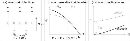
Ferrimagnetism combines antiparallel order with an uncompensated moment. Different sublattice temperature dependences can cross at $T_M$ while both remain ordered until $T_C$. An ideal two-sublattice ferrimagnet supports a gapless acoustic branch and a gapped optical branch; their detailed dispersions and gaps depend on exchange, anisotropy, field, and lattice geometry.

Angular-Momentum Compensation

Magnetization and angular momentum are not the same quantity when sublattices have different gyromagnetic ratios. Let $\gamma_A$ and $\gamma_B$ denote positive gyromagnetic-ratio magnitudes. The signed net angular-momentum density is proportional to

$$\mathcal J_{\mathrm{net}} = \frac{M_A}{\gamma_A} - \frac{M_B}{\gamma_B}.$$

The angular-momentum compensation temperature $T_A$ satisfies

$$\frac{ M_A(T_A) }{\gamma_A} = \frac{ M_B(T_A) }{\gamma_B}.$$

If $\gamma_A=\gamma_B$, then $T_A=T_M$. Otherwise the two temperatures generally differ.

At $T_M$, the magnetic moment vanishes but the net spin angular momentum can remain nonzero. At $T_A$, the net angular momentum vanishes while the magnetic moment can remain nonzero. This distinction is essential in rare-earth–transition-metal ferrimagnets, where the sublattice $g$ factors and orbital contributions differ.

The broken spin generators obey

$$\left[ S^x_{\mathrm{tot}}, S^y_{\mathrm{tot}} \right] = i\hbar S^z_{\mathrm{tot}}.$$

Their commutator expectation is controlled by net angular momentum, not directly by net magnetization. Away from $T_A$, an isotropic ferrimagnet has ferromagnetic-like type-B low-energy dynamics. Near $T_A$, the leading gyrotropic term can vanish and the dynamics becomes antiferromagnetic-like. Damping, inertia, anisotropy, and mode hybridization still remain material dependent.

Collective Modes

Two coupled sublattices produce at least two characteristic precession patterns:

• an acoustic mode, in which the sublattices remain nearly antiparallel while the common axis varies slowly;
• an optical mode, in which the relative angle oscillates strongly against the intersublattice exchange.

The names describe low-energy character, not light coupling. A complex ferrite with many magnetic ions in its primitive cell has many optical branches.

Alternating-spin-chain benchmark

Consider a one-dimensional cell of length $a$ with spins $S_A>S_B$, antiferromagnetic exchange $J>0$, and bonds $A_n$–$B_n$ and $B_n$–$A_{n+1}$. Linear spin-wave theory gives

$$\hbar\omega_\pm(k) = J \left[ \sqrt{ \left( S_A-S_B \right)^2 + 4S_AS_B \sin^2 \left( \frac{ka}{2} \right) } \pm \left( S_A-S_B \right) \right].$$

The lower branch is

$$\hbar\omega_-(0) = 0,$$

while the optical gap is

$$\hbar\omega_+(0) = 2J \left( S_A-S_B \right).$$

At small $k$,

$$\hbar\omega_-(k) \simeq \frac{ JS_AS_Ba^2 }{ 2(S_A-S_B) } k^2.$$

The quadratic Goldstone branch reflects nonzero net spin per cell. In the compensated limit $S_A\to S_B$, the two branches become degenerate and linear at small $k$, recovering antiferromagnetic mode structure.

This exactly stated chain result is a benchmark, not a universal fit for a three-dimensional ferrite. Real dispersions include many exchange paths, anisotropy gaps, dipolar mixing, noncollinearity, damping, and magnon–phonon hybridization.

Opposite spin carried by the branches

Acoustic and optical magnons can carry opposite angular momentum relative to the ordered state. Their thermal populations can therefore reduce different sublattice contributions at different rates and help produce compensation. In multi-branch materials, the sign and magnitude of magnon spin can depend on wavevector and mode mixing.

Ferrites

Ferrites are iron-containing oxides whose magnetic ions occupy multiple crystallographic sublattices. Many are ferrimagnetic electrical insulators. Oxygen-mediated superexchange commonly aligns important sublattice moments antiparallel, while site occupancy determines the residual moment.

The name “ferrite” is chemical and structural, not a guarantee of one ideal magnetic model. Cation disorder, vacancies, mixed valence, canting, finite particle size, and secondary phases can strongly alter the magnetization.

Spinel ferrites

Spinels have ideal composition

$$AB_2O_4$$

with tetrahedral and octahedral cation sites. Crystallographic notation often uses parentheses for tetrahedral occupancy and brackets for octahedral occupancy.

A normal spinel places the divalent cation on tetrahedral sites and trivalent cations on octahedral sites. An inverse spinel exchanges part of that occupancy. The inversion parameter, valence state, and site-specific exchange determine the magnetic structure.

For ideal inverse-spinel magnetite,

$$\left( \mathrm{Fe}^{3+} \right)_A \left[ \mathrm{Fe}^{3+} \mathrm{Fe}^{2+} \right]_B O_4.$$

High-spin $\mathrm{Fe}^{3+}$ contributes approximately $5\mu_{\mathrm B}$ and high-spin $\mathrm{Fe}^{2+}$ approximately $4\mu_{\mathrm B}$ in spin-only ionic counting. The opposing $\mathrm{Fe}^{3+}$ moments cancel, leaving

$$\mu_{\mathrm{ideal}} \simeq 4\mu_{\mathrm B}$$

per formula unit. Magnetite also has mixed-valence electronic and structural physics, including the low-temperature Verwey transition, so the ionic picture is a starting ledger rather than a complete theory.

Garnets

Yttrium iron garnet,

$$\mathrm{Y}_3 \mathrm{Fe}_5 \mathrm O_{12},$$

contains nonmagnetic $\mathrm Y^{3+}$ and high-spin $\mathrm{Fe}^{3+}$ on inequivalent octahedral and tetrahedral sites. In ideal collinear counting, two $\mathrm{Fe}^{3+}$ moments on one sublattice oppose three on the other, giving

$$\mu_{\mathrm{ideal}} \simeq 5\mu_{\mathrm B}$$

per formula unit at zero temperature.

YIG is a ferrimagnetic insulator with low magnetic damping in high-quality samples. Its many magnetic sites produce a rich magnon spectrum; treating it as a one-spin ferromagnet is adequate only in a restricted long-wavelength window.

Rare-earth iron garnets

$$R_3 \mathrm{Fe}_5 \mathrm O_{12}$$

add a magnetic rare-earth sublattice. The rare-earth and iron sublattices can have very different thermal dependences, making compensation and spin-reorientation phenomena common.

Hexaferrites

Hexaferrites such as barium hexaferrite contain several inequivalent Fe sites and strong magnetocrystalline anisotropy. Their large coercivity and chemical stability support permanent-magnet and microwave uses. Simple two-sublattice counting can organize the net moment, but quantitative modeling requires the full site occupancy and exchange network.

Other Ferrimagnetic Platforms

Rare-earth–transition-metal alloys

Amorphous alloys such as GdFeCo combine a rare-earth $4f$ sublattice with an antiferromagnetically coupled transition-metal $3d$ sublattice. Their different moments, $g$ factors, and demagnetization times separate $T_M$ from $T_A$ and enable element-resolved ultrafast dynamics.

After strong optical excitation, the two sublattices need not remain rigidly antiparallel at every instant. A transient nearly parallel configuration can occur during reversal. This is a nonequilibrium pathway, not a new equilibrium ferromagnetic phase.

Molecular and low-dimensional ferrimagnets

Alternating-spin chains, coordination compounds, and molecular magnets can realize unequal sublattice spins with clean model Hamiltonians. In one dimension, quantum and thermal fluctuations prevent the same finite-temperature long-range order expected in three-dimensional bulk ferrites unless anisotropy, long-range coupling, or interchain interactions intervene.

Synthetic ferrimagnets

Two ferromagnetic layers coupled antiferromagnetically through a spacer form a synthetic ferrimagnet when their areal moments are unequal. This engineered structure shares net and staggered variables with atomic ferrimagnets but has mesoscopic layer degrees of freedom, interfacial exchange, and distinct domain-wall physics.

Domains and Hysteresis

Because $M_{\mathrm{net}}\ne0$ away from compensation, a ferrimagnet produces magnetostatic fields and can form flux-reducing domains. Its low-frequency hysteresis can look ferromagnetic:

• remanence follows domain populations;
• coercivity depends on pinning and anisotropy;
• saturation aligns the net moment and can also modify canting;
• loop area measures protocol-dependent dissipation.

The internal sublattice order cannot be inferred from the loop alone. A ferromagnet, ferrimagnet, canted antiferromagnet, and multiphase sample can all show a net hysteretic moment.

Near $T_M$, the small net moment reduces Zeeman and magnetostatic energies while anisotropy can remain finite. Domain selection by a field may therefore become difficult, and coercive fields can change sharply. A vanishing bulk loop can also result from equal domain populations, so compensation requires sublattice-resolved evidence or a reproducible intrinsic zero crossing.

Experimental Identification

Bulk magnetometry

Measure $M(H,T)$ with background subtraction, demagnetizing correction, and a declared field-cooling protocol. A ferrimagnetic candidate should show an ordered state with a saturation moment inconsistent with simple parallel alignment of all magnetic ions.

A compensation point is strengthened by:

• a signed magnetization reversal in a pinned or exchange-biased domain;
• a reproducible minimum in high-field net magnetization;
• element- or site-resolved sublattice moments crossing;
• persistence of magnetic diffraction and local fields through $T_M$;
• absence of a thermodynamic singularity unless another transition coincides.

Diffraction and local probes

Neutron diffraction can refine antiparallel moments on crystallographic sites. Magnetic x-ray diffraction, x-ray magnetic circular dichroism, and x-ray magnetic linear dichroism can isolate elements and, in favorable cases, sites or orbital contributions.

Mössbauer spectroscopy is especially valuable for Fe-containing ferrites because hyperfine fields and valence-sensitive shifts distinguish inequivalent iron environments. Nuclear magnetic resonance and muon spin rotation provide complementary local-field and dynamic information.

Dynamic spectroscopy

Ferromagnetic resonance, broadband microwave spectroscopy, Brillouin light scattering, inelastic neutron scattering, and time-resolved magneto-optics can separate acoustic and optical modes. A credible mode assignment uses:

• field and temperature dependence;
• polarization and selection rules;
• spectral weight on each sublattice;
• wavevector dispersion;
• comparison with the full exchange and anisotropy model.

An optical branch can be weak in a probe that couples mainly to net magnetization. Its absence from one spectrum does not prove that the sublattice degree of freedom is absent.

Applications and Material Tradeoffs

Soft ferrites

Mn–Zn and Ni–Zn ferrites combine magnetic permeability with high electrical resistivity. In transformer cores, inductors, and electromagnetic-interference components, the resistivity suppresses eddy-current loss relative to a conducting metal. Frequency range, saturation flux density, temperature stability, porosity, and hysteretic loss still impose tradeoffs.

Hard ferrites

Barium and strontium hexaferrites have strong anisotropy and substantial coercivity. They are used as chemically stable, rare-earth-free permanent magnets and magnetic-recording materials. Their energy product is lower than that of leading rare-earth magnets, so “rare-earth free” does not mean performance-equivalent in every geometry.

Microwave nonreciprocity

A biased ferrimagnet has a tensor magnetic susceptibility with off-diagonal gyrotropic components. Ferrite circulators, isolators, phase shifters, and tunable filters exploit this nonreciprocity. Device behavior depends on bias field, resonance linewidth, geometry, dielectric loss, and temperature.

Magnonics and spin transport

High-quality YIG supports long-lived spin waves over selected frequency and wavevector ranges. It is widely used to study magnon transport, spin pumping, magnon–photon coupling, and spin caloritronics.

Low damping is sample-, thickness-, interface-, and mode-dependent. Patterning, surface damage, rare-earth impurities, two-magnon scattering, and adjacent metals can broaden the linewidth.

Ultrafast and compensation-point dynamics

Rare-earth–transition-metal ferrimagnets support ultrafast optical and current-driven reversal. Near $T_A$, reduced net angular momentum can increase domain-wall mobility and alter precession.

These results are material- and protocol-specific. A short laser pulse also heats electrons and lattices, changes anisotropy, and drives the system far from equilibrium. Switching claims require element-resolved timing, fluence dependence, thermal modeling, and separation of helicity-dependent from purely thermal mechanisms.

Distinguishing Nearby Magnetic States

State	Sublattice relation	Net moment	Defining distinction
Ferromagnet	Moments align in the primary order	Nonzero	Uniform magnetization is primary
Collinear antiferromagnet	Equivalent opposing sublattices	Zero ideally	Compensation follows symmetry equivalence
Ferrimagnet	Inequivalent opposing sublattices	Usually nonzero	Net moment is an intrinsic difference
Canted antiferromagnet	Nearly equivalent opposing sublattices	Small secondary moment	Canting, often from anisotropic exchange
Compensated ferrimagnet at $T_M$	Inequivalent ordered sublattices	Zero at one temperature	Sublattice order remains nonzero
Synthetic ferrimagnet	Opposing magnetic layers	Tunable	Mesoscopic layer moments replace atomic sublattices
Multiphase mixture	Distinct magnetic phases coexist	Variable	No single homogeneous sublattice order

The magnetic structure and site-resolved moments decide the classification. Net magnetization alone does not.

Reliable Analysis Workflow

1. List magnetic sites and occupancies. Include valence, coordination, multiplicity, and disorder.
2. Fix the sign ledger. Define sublattice directions, vector versus positive magnitudes, and factors of $1/2$.
3. Count the ionic baseline. Then state covalency, orbital, itinerant, and noncollinear corrections.
4. Determine the structure. Use diffraction or site-resolved spectroscopy to establish antiparallel inequivalent sublattices.
5. Track each sublattice with temperature. Net magnetometry cannot locate the microscopic crossing by itself.
6. Separate $T_M$, $T_A$, and $T_C$. Report how each was measured.
7. Resolve acoustic and optical modes. Fit dispersion and spectral weight, not only one resonance.
8. Control domains and secondary phases. Check cooling history, particle size, interfaces, and chemical homogeneity.
9. Match applications to loss channels. Quote damping, coercivity, resistivity, thermal stability, and geometry under operating conditions.

Common mistakes

• Calling ferrimagnetism a weak form of ferromagnetism.
• Defining it only by a nonzero net moment.
• Confusing magnetization compensation with loss of magnetic order.
• Assuming $T_M=T_A$ without checking $g$ factors.
• Calling a compensated ferrimagnet an antiferromagnet without specifying symmetry and sublattice inequivalence.
• Treating every ferrite as an ideal collinear two-sublattice magnet.
• Using nominal chemistry instead of measured cation occupancy.
• Inferring site moments from bulk saturation alone.
• Ignoring optical magnon branches in a multi-sublattice crystal.
• Applying one Curie–Weiss fit across a curved inverse susceptibility.
• Interpreting a low-field zero as compensation without excluding domains.
• Generalizing low damping or ultrafast switching from one optimized material to all ferrimagnets.

Exercises

1. Net and staggered components

Let

$$\mathbf M_A = M_A\mathbf n, \qquad \mathbf M_B = -M_B\mathbf n,$$

with $M_A>M_B>0$. Compute $\mathbf M$ and $\mathbf L$ using the half-sum convention, and repeat at a compensation point.

Solution

The uniform component is

$$\mathbf M = \frac{ \mathbf M_A+\mathbf M_B }{2} = \frac{ M_A-M_B }{2} \mathbf n.$$

The staggered component is

$$\mathbf L = \frac{ \mathbf M_A-\mathbf M_B }{2} = \frac{ M_A+M_B }{2} \mathbf n.$$

At compensation, $M_A=M_B=M_0$, so

$$\mathbf M = \mathbf0, \qquad \mathbf L = M_0\mathbf n.$$

The calculation makes explicit that compensation removes only the uniform combination.

2. Ionic counting in magnetite

Use ideal inverse-spinel magnetite,

$$\left( \mathrm{Fe}^{3+} \right)_A \left[ \mathrm{Fe}^{3+} \mathrm{Fe}^{2+} \right]_B O_4,$$

with spin-only moments $5\mu_{\mathrm B}$ for $\mathrm{Fe}^{3+}$ and $4\mu_{\mathrm B}$ for $\mathrm{Fe}^{2+}$. Find the net moment per formula unit.

Solution

The $A$-site $\mathrm{Fe}^{3+}$ moment is antiparallel to the two $B$-site moments. Therefore

$$\begin{aligned} \mu_{\mathrm{net}} &= \left| \left( 5+4 \right) - 5 \right| \mu_{\mathrm B} \\ &= 4\mu_{\mathrm B}. \end{aligned}$$

The two $\mathrm{Fe}^{3+}$ contributions cancel in the ideal ionic picture. A measured deviation can reflect covalency, canting, nonstoichiometry, finite temperature, or an incorrect site-occupancy model.

3. A compensation temperature

Suppose the sublattice magnitudes are modeled for $0<T<T_C$ by

$$M_A(T) = M_{A0} \left( 1-\frac{T}{T_C} \right)^{1/2},$$

and

$$M_B(T) = M_{B0} \left( 1-\frac{T}{T_C} \right)^{1/3},$$

with $M_{A0}>M_{B0}$. Find the condition for a compensation point and its temperature.

Solution

Set $x=1-T/T_C$. Compensation requires

$$M_{A0}x^{1/2} = M_{B0}x^{1/3}.$$

For $x>0$,

$$x^{1/6} = \frac{ M_{B0} }{M_{A0}},$$

so

$$x = \left( \frac{ M_{B0} }{M_{A0}} \right)^6.$$

Therefore

$$T_M = T_C \left[ 1 - \left( \frac{ M_{B0} }{M_{A0}} \right)^6 \right].$$

Because $0<M_{B0}/M_{A0}<1$, this lies strictly between zero and $T_C$. The powers are phenomenological; the exercise illustrates how different thermal curves can cross.

4. Magnetization versus angular-momentum compensation

At some temperature, let

$$M_A = 1.00 \quad\text{and}\quad M_B = 0.90$$

in common units, with $g_A=2.00$ and $g_B=1.80$. Is the system at magnetization compensation or angular-momentum compensation if $\gamma_\alpha\propto g_\alpha$?

Solution

Magnetization compensation would require $M_A=M_B$, which is false:

$$M_A-M_B = 0.10.$$

For angular momentum,

$$\frac{M_A}{g_A} = \frac{1.00}{2.00} = 0.50,$$

and

$$\frac{M_B}{g_B} = \frac{0.90}{1.80} = 0.50.$$

Thus the net angular momentum vanishes while the net magnetization remains nonzero. This is an angular-momentum compensation point but not a magnetization compensation point.

5. Ferrimagnetic spin-wave limits

For the alternating-spin-chain dispersion

$$\hbar\omega_\pm(k) = J \left[ \sqrt{ \Delta S^2 + 4S_AS_B \sin^2 \left( \frac{ka}{2} \right) } \pm \Delta S \right],$$

where $\Delta S=S_A-S_B>0$, derive the optical gap and the leading small-$k$ acoustic dispersion.

Solution

At $k=0$, the square root is $\Delta S$, so

$$\hbar\omega_-(0) = 0$$

and

$$\hbar\omega_+(0) = 2J\Delta S.$$

For small $k$,

$$4S_AS_B \sin^2 \left( \frac{ka}{2} \right) \simeq S_AS_Bk^2a^2.$$

Expanding the square root,

$$\sqrt{ \Delta S^2 + S_AS_Bk^2a^2 } \simeq \Delta S + \frac{ S_AS_Bk^2a^2 }{ 2\Delta S }.$$

Therefore

$$\hbar\omega_-(k) \simeq \frac{ JS_AS_Ba^2 }{ 2\Delta S } k^2.$$

The expansion fails as $\Delta S\to0$ because the compensated antiferromagnetic limit is linear rather than quadratic.

6. Lieb–Mattis spin for an unequal bipartite cell

A bipartite cluster contains four spin-$1$ sites on $A$ and six spin-$1/2$ sites on $B$, with only antiferromagnetic intersublattice couplings satisfying the Lieb–Mattis assumptions. Find the ground-state total spin.

Solution

The maximal sublattice spins are

$$S_A^{\max} = 4,$$

and

$$S_B^{\max} = 6 \left( \frac12 \right) = 3.$$

Hence

$$S_{\mathrm{tot}} = \left| 4-3 \right| = 1.$$

The ground state is a spin-one multiplet rather than a singlet. This is a finite-system quantum signature of sublattice imbalance under the theorem’s assumptions.

7. Compensation or domains?

A sample’s low-field magnetization crosses zero at $180\,\mathrm K$, but its high-field magnetization remains positive and element-resolved x-ray signals do not cross. Magnetic imaging shows equal up and down domains near that temperature. Is a compensation point established?

Solution

No. Equal domain populations can cancel the low-field bulk moment without equality of the sublattice magnitudes. The positive high-field moment and absence of an element-resolved crossing argue against intrinsic magnetization compensation.

A stronger test would track signed, sublattice-resolved moments through the candidate temperature under a domain-pinning or exchange-bias protocol. Magnetic diffraction should confirm that order persists, while high-field net magnetization should approach an intrinsic minimum or zero after backgrounds and canting are treated.

Connections

• Exchange Interactions derives the antiferromagnetic and anisotropic couplings that organize ferrimagnetic sublattices.
• Ferromagnetism owns spontaneous uniform magnetization, domains, hysteresis, and ferromagnetic spin-wave scaling.
• Antiferromagnetism develops compensated staggered order, spin flop, frustration, and antiferromagnetic type-A modes.
• Magnetic Anisotropy develops easy directions, demagnetizing geometry, interface terms, and the texture scales relevant to ferrites and compensated films.
• Heisenberg Model supplies bipartite exchange conventions and quantum finite-size benchmarks.
• Magnons owns the bosonic quantization, spectral weights, damping, and validity tests behind acoustic and optical branches.
• Spin Waves and Magnons in Materials connects multi-sublattice order to acoustic and optical intensities, compensation dynamics, linewidths, and material-model tests.
• Spintronics develops spin pumping, inverse detection, current-induced torque, and the device tradeoffs behind ferrimagnetic and magnetic-insulator platforms.
• Skyrmions and Magnetic Textures connects angular-momentum compensation to texture gyroforces, transverse drift, and stability.
• Magnetic Moments and g-Factors distinguishes magnetic moment from angular momentum and fixes gyromagnetic conventions.
• Hund’s Rules provides the atomic baseline used in ideal ionic moment counting.
• Finite-Temperature Phase Transitions distinguishes a true $T_C$ singularity from compensation inside an ordered phase.
• Hall Effect gives the symmetry and scaling tests for ordinary and anomalous transverse signals in magnetic materials.
• Condensed-Matter Roadmap places ferrimagnetism between exchange, collective modes, materials, and devices.

References

1. L. Néel, “Propriétés magnétiques des ferrites; ferrimagnétisme et antiferromagnétisme,” Annales de Physique 12, 137–198 (1948), doi:10.1051/anphys/194812030137.
2. Y. Yafet and C. Kittel, “Antiferromagnetic Arrangements in Ferrites,” Physical Review 87, 290–294 (1952), doi:10.1103/PhysRev.87.290.
3. E. Lieb and D. Mattis, “Ordering Energy Levels of Interacting Spin Systems,” Journal of Mathematical Physics 3, 749–751 (1962), doi:10.1063/1.1724276.
4. S. Geller and M. A. Gilleo, “Structure and Ferrimagnetism of Yttrium and Rare-Earth–Iron Garnets,” Acta Crystallographica 10, 239 (1957), doi:10.1107/S0365110X57000729.
5. J. Smit and H. P. J. Wijn, Ferrites (Philips Technical Library, 1959).
6. V. Cherepanov, I. Kolokolov, and V. L’vov, “The Saga of YIG: Spectra, Thermodynamics, Interaction and Relaxation of Magnons in a Complex Magnet,” Physics Reports 229, 81–144 (1993), doi:10.1016/0370-1573(93)90107-O.
7. J. M. D. Coey, Magnetism and Magnetic Materials (Cambridge University Press, 2010), doi:10.1017/CBO9780511845000.
8. B. Hillebrands and A. Thiaville, eds., Spin Dynamics in Confined Magnetic Structures III (Springer, 2006), doi:10.1007/10938171.
9. C. D. Stanciu et al., “All-Optical Magnetic Recording with Circularly Polarized Light,” Physical Review Letters 99, 047601 (2007), doi:10.1103/PhysRevLett.99.047601.
10. I. Radu et al., “Transient Ferromagnetic-Like State Mediating Ultrafast Reversal of Antiferromagnetically Coupled Spins,” Nature 472, 205–208 (2011), doi:10.1038/nature09901.
11. K.-J. Kim et al., “Fast Domain Wall Motion in the Vicinity of the Angular Momentum Compensation Temperature of Ferrimagnets,” Nature Materials 16, 1187–1192 (2017), doi:10.1038/nmat4990.
12. A. V. Chumak et al., “Magnon Spintronics,” Nature Physics 11, 453–461 (2015), doi:10.1038/nphys3347.
13. Y. Kajiwara et al., “Transmission of Electrical Signals by Spin-Wave Interconversion in a Magnetic Insulator,” Nature 464, 262–266 (2010), doi:10.1038/nature08876.
14. A. Kirilyuk, A. V. Kimel, and T. Rasing, “Ultrafast Optical Manipulation of Magnetic Order,” Reviews of Modern Physics 82, 2731–2784 (2010), doi:10.1103/RevModPhys.82.2731.
15. R. L. Stamps et al., “The 2014 Magnetism Roadmap,” Journal of Physics D: Applied Physics 47, 333001 (2014), doi:10.1088/0022-3727/47/33/333001.