Stoner Criterion

The Stoner criterion is the local mean-field stability test for a spatially uniform, unpolarized metal against an infinitesimal spin polarization. In a scalar one-band convention with density of states per spin $N(E_{\mathrm F})$ and Stoner interaction $I$, the paramagnetic state loses quadratic stability when

$$I\,N(E_{\mathrm F}) > 1.$$

The compact inequality is useful only after its ledger is fixed. Whether $N$ is per spin or spin summed, per atom or per volume, and whether $I$ multiplies particle-number polarization or magnetic moment all change the symbols appearing in the formula. A factor-of-two error can turn a strongly enhanced paramagnet into a claimed ferromagnet.

This page is the canonical home for:

• the scalar energy-curvature derivation of the criterion;
• the equivalent susceptibility derivation;
• the finite-temperature thermal density of states;
• nonlinear stabilization when the density of states varies with energy;
• practical extraction of a Stoner enhancement or curvature;
• the distinction between a local instability test and a material diagnosis.

Itinerant Magnetism owns exchange-split bands, spin-density waves, the Stoner continuum, and experimental material classification. Random Phase Approximation owns the general response resummation and matrix pole condition. Ferromagnetism owns the ordered phase, domains, thermodynamics, and local-moment comparison.

Required background. Density of States supplies the per-spin state-counting convention, while Mean-Field Theory supplies the self-consistent closure and local-stability logic.

Helpful background. Itinerant Magnetism supplies the material and exchange-split band context. Fermi Surface and Susceptibilities provide the geometric and response tools for extensions.

Assumptions Before the Algebra

The textbook criterion assumes:

1. a metallic paramagnetic reference state;
2. a rigid spin-degenerate band structure for the kinetic-energy estimate;
3. a uniform collinear polarization;
4. a static, momentum-independent effective interaction;
5. a mean-field treatment of that interaction;
6. an expansion about zero polarization;
7. a density of states smooth enough for the chosen expansion.

Relaxing these assumptions can change the instability wavevector, transition order, ordered moment, transition temperature, or even the appropriate low-energy variables. The criterion is therefore a controlled statement inside a model, not a theorem that every large-density-of-states metal must become ferromagnetic.

What “local stability” means

Let $m$ denote the spin-population difference in a fixed normalization unit. If the zero-field energy is

$$E(m) = E(0) + a_2m^2 + a_4m^4 + \cdots,$$

then the unpolarized state is locally stable when $a_2>0$ and locally unstable when $a_2<0$. The Stoner criterion determines the sign of $a_2$ in the simplest rigid-band mean field.

It does not by itself determine the global minimum. If $a_4<0$ and a positive sixth-order term stabilizes the energy, a finite-$m$ state can become globally favorable while $m=0$ remains locally stable. That is a first-order transition, and its coexistence point need not satisfy $I N(E_{\mathrm F})=1$.

Convention Ledger

Density of states per spin

Let

$$N(\varepsilon) = \frac{1}{\mathcal V} \sum_{n,\mathbf k} \delta( \varepsilon-\varepsilon_{n\mathbf k} )$$

denote the density of states for one spin species in the unpolarized reference. The normalization unit $\mathcal V$ may be a physical volume, a primitive cell, an atom, or a formula unit. The interaction parameter must use the same unit.

The spin-summed density of states is

$$N_{\mathrm{tot}}(\varepsilon) = 2N(\varepsilon)$$

when spin degeneracy is intact. With the interaction convention used below,

$$I\,N(E_{\mathrm F})>1$$

is equivalent to

$$I\,N_{\mathrm{tot}}(E_{\mathrm F})>2.$$

Writing $I N_{\mathrm{tot}}>1$ without redefining $I$ is the common factor-of-two mistake.

Polarization and magnetic moment

Define

$$m := n_\uparrow-n_\downarrow, \qquad n = n_\uparrow+n_\downarrow.$$

Here $m$ is a particle-number difference, not yet a magnetic moment. Let

$$\mu_s = \frac{g\mu_B}{2}$$

be the magnitude of the magnetic moment associated with one unit of spin-population imbalance. The spin magnetization is then

$$M_s = \mu_s m.$$

For $g\simeq2$, $\mu_s\simeq\mu_B$. In tables that quote a moment in $\mu_B$ per atom, the numerical values of $m$ and $M_s/\mu_B$ may coincide, but their dimensions and definitions do not.

Interaction parameter

Use the scalar interaction energy

$$E_{\mathrm{int}} = I\,n_\uparrow n_\downarrow.$$

At fixed $n$,

$$n_\uparrow = \frac{n+m}{2}, \qquad n_\downarrow = \frac{n-m}{2},$$

so

$$\Delta E_{\mathrm{int}} = - \frac{I}{4}m^2.$$

In a single-band Hubbard mean field, $I$ can coincide with the on-site parameter $U$ under a matching normalization. In a multiorbital material or density-functional calculation, an effective Stoner parameter contains orbital projection and exchange-correlation information. It should not be identified automatically with a bare Coulomb integral.

Derivation from Spin Transfer

Transfer at fixed total density

Begin with equal spin populations and transfer

$$x = \frac{m}{2}$$

particles from the down-spin Fermi sea to the up-spin Fermi sea. The total density remains fixed:

$$\delta n_\uparrow = x, \qquad \delta n_\downarrow = -x.$$

Near the Fermi energy, take the one-spin density of states to be locally constant:

$$N(\varepsilon) \simeq N(E_{\mathrm F}).$$

Adding $x$ particles raises one spin-resolved Fermi edge by

$$\delta\varepsilon_\uparrow = \frac{x}{N(E_{\mathrm F})},$$

while removing $x$ particles lowers the other by the same amount.

Band-energy cost

The incremental energy to transfer an additional amount $dx'$ grows linearly with the separation of the two spin-resolved Fermi edges. Integrating both contributions gives

$$\begin{aligned} \Delta E_{\mathrm{band}} &= 2 \int_0^x \frac{x'}{N(E_{\mathrm F})} \,dx' \\ &= \frac{x^2}{N(E_{\mathrm F})} \\ &= \frac{m^2}{ 4N(E_{\mathrm F}) }. \end{aligned}$$

This is the Pauli cost of making two Fermi seas unequal. A large density of states makes the cost small because many states are available within a narrow energy interval.

Exchange-energy gain

The interaction contribution found above is

$$\Delta E_{\mathrm{int}} = - \frac{I}{4}m^2.$$

The minus sign does not mean that every repulsive interaction favors bulk ferromagnetism. It means that, within this mean-field decoupling, polarization reduces the probability of opposite-spin occupancy and therefore lowers the interaction energy.

Total curvature

Combining the two pieces,

$$\Delta E(m) = \frac{m^2}{4} \left[ \frac{1}{N(E_{\mathrm F})} - I \right] + O(m^4).$$

The curvature at the origin is

$$\left. \frac{d^2E}{dm^2} \right|_{m=0} = \frac12 \left[ \frac{1}{N(E_{\mathrm F})} - I \right].$$

Therefore:

Stoner product	Quadratic curvature	Scalar mean-field conclusion
$I N(E_{\mathrm F})<1$	positive	unpolarized state locally stable
$I N(E_{\mathrm F})=1$	zero	marginal at quadratic order
$I N(E_{\mathrm F})>1$	negative	unpolarized state locally unstable

The instability condition is

$$I\,N(E_{\mathrm F}) > 1.$$

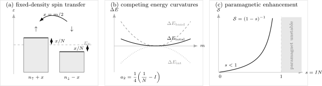
The scalar Stoner ledger. A fixed-density transfer $m/2$ separates the two spin-resolved Fermi edges. Band filling gives positive curvature $1/N(E_{\mathrm F})$, exchange gives negative curvature $-I$, and the paramagnetic susceptibility enhancement $\mathcal S=[1-I N(E_{\mathrm F})]^{-1}$ diverges on approaching the mean-field threshold from below. The shaded side is not described by the paramagnetic response formula.

Derivation from Susceptibility

The same condition follows from the response to a uniform magnetic source.

Couple an external field

For a weak induction $B$, the spin Zeeman energy is

$$\Delta E_B = - \mu_s Bm.$$

To quadratic order,

$$\Delta E(m;B) = \frac{m^2}{4} \left[ \frac{1}{N(E_{\mathrm F})} - I \right] - \mu_s Bm.$$

Minimizing with respect to $m$ gives

$$m = \frac{ 2\mu_s N(E_{\mathrm F}) }{ 1-I N(E_{\mathrm F}) } B.$$

Pauli susceptibility and enhancement

If $m$ and $N$ are normalized per physical volume, then $M_s=\mu_s m$ and $B\simeq\mu_0H$ in the source term. The dimensionless SI spin susceptibility is

$$\chi_s := \frac{\partial M_s}{\partial H} = \frac{ 2\mu_0\mu_s^2N(E_{\mathrm F}) }{ 1-I N(E_{\mathrm F}) }.$$

The noninteracting Pauli value in this convention is

$$\chi_{\mathrm P} = 2\mu_0\mu_s^2N(E_{\mathrm F}),$$

so the Stoner enhancement is

$$\mathcal S := \frac{\chi_s}{\chi_{\mathrm P}} = \frac{1}{ 1-I N(E_{\mathrm F}) }.$$

For a stable paramagnet,

$$I N(E_{\mathrm F}) = 1-\frac{1}{\mathcal S}.$$

The enhancement formula is a response about $m=0$. Continuing it to $I N>1$ and reporting a negative paramagnetic susceptibility is not a physical prediction; it is the signal that the assumed reference state is unstable.

Equality is not a complete transition theory

At $I N=1$, the scalar mean-field inverse susceptibility vanishes and the quadratic energy is flat. Higher-order band curvature, finite temperature, nonuniform channels, anisotropy, disorder, and fluctuations then matter. The equality marks a local mean-field boundary, not automatically an experimentally observed continuous critical point.

Self-Consistent Exchange Splitting

The curvature argument can be written as a self-consistency equation.

Splitting convention

Let the spin-resolved quasiparticle energies be shifted by

$$\varepsilon_{\mathbf k\uparrow} = \varepsilon_{\mathbf k} - \frac{\Delta}{2}, \qquad \varepsilon_{\mathbf k\downarrow} = \varepsilon_{\mathbf k} + \frac{\Delta}{2},$$

with

$$\Delta = I m + 2\mu_s B.$$

The factor of two in the Zeeman contribution appears because $\Delta$ is the full separation between the two spin energies.

Nonlinear equation

For a rigid one-spin density of states,

$$\begin{aligned} m = \int d\varepsilon\, N(\varepsilon) \Big[ & f( \varepsilon-\mu-\Delta/2 ) \\ - & f( \varepsilon-\mu+\Delta/2 ) \Big]. \end{aligned}$$

At zero field, a nonzero solution must satisfy this equation together with $\Delta=Im$ and the fixed-density condition. Linearizing in $\Delta$ gives

$$m = N_T(\mu,T)\Delta + O(\Delta^3),$$

where $N_T$ is the thermally averaged density of states defined below. A nonzero infinitesimal solution appears when

$$I N_T(\mu,T) = 1.$$

Why a constant density of states does not fix the moment

An exactly constant, infinitely wide density of states makes both the band cost and exchange gain purely quadratic. Above threshold the truncated energy has negative curvature but no stabilizing scale. The model then says that $m=0$ is unstable without determining the new minimum.

The ordered moment comes from information absent from the criterion:

• band edges and total filling;
• energy dependence of the density of states;
• orbital-dependent exchange;
• self-consistent changes of the bands;
• higher-order interaction and correlation effects.

The inequality predicts the loss of stability, not the magnitude of the resulting magnetization.

Finite Temperature

Thermal density of states

At temperature $T$, the Fermi edge is broadened. Define

$$N_T(\mu,T) := \int_{-\infty}^{\infty} d\varepsilon\, N(\varepsilon) \left[ - \frac{\partial f( \varepsilon-\mu )}{\partial\varepsilon} \right].$$

The kernel is positive, normalized, and concentrated within an energy window of order $k_{\mathrm B}T$ around $\mu$. At zero temperature,

$$\lim_{T\to0} N_T(\mu,T) = N(E_{\mathrm F}).$$

The finite-temperature scalar condition is

$$I N_T( \mu(T),T_C ) = 1.$$

At fixed particle number, $\mu(T)$ is determined from the number equation. Its first-order change under an infinitesimal spin splitting cancels between the two spin species, but its ordinary temperature dependence must still be included.

Smooth-density expansion

If $N(\varepsilon)$ is smooth on the thermal scale, the Sommerfeld expansion gives

$$\begin{aligned} N_T(\mu,T) = & N(\mu) \\ & + \frac{\pi^2}{6} (k_{\mathrm B}T)^2 N''(\mu) + O(T^4). \end{aligned}$$

Thermal smearing can either raise or lower the averaged density of states depending on local curvature and on the shift of $\mu(T)$. Near a sharp van Hove feature, this smooth expansion may fail and the integral definition should be used directly.

Mean-field Curie–Weiss form

On the paramagnetic side,

$$\chi_s(T) = \frac{ \chi_{\mathrm P}(T) }{ 1-I N_T(T) }.$$

If $N_T(T)$ crosses $1/I$ smoothly and its derivative at $T_C$ is nonzero, then

$$1-I N_T(T) \simeq - I \left. \frac{dN_T}{dT} \right|_{T_C} (T-T_C),$$

which produces a mean-field Curie–Weiss-like pole. Its slope is controlled by the thermally averaged band structure in this model.

An infinitely wide constant density of states has $N_T=N$ and therefore supplies no temperature scale at all. A finite $T_C$ requires band structure, self-consistency, or physics beyond that caricature. There is no universal rule that converts $I N(E_{\mathrm F})-1$ directly into a reliable material Curie temperature.

Energy-Dependent Density of States

The quadratic criterion can be extended systematically for a smooth rigid band.

Fixed-density expansion

Write

$$N_j := \left. \frac{d^jN}{d\varepsilon^j} \right|_{E_{\mathrm F}}, \qquad N_0 = N(E_{\mathrm F}).$$

At zero temperature, transfer $m/2$ particles between spin species while keeping the total density fixed. Series inversion of the number integrals gives

$$\begin{aligned} \Delta E_{\mathrm{band}} = & \frac{m^2}{4N_0} \\ & + \left[ \frac{N_1^2}{64N_0^5} - \frac{N_2}{192N_0^4} \right] m^4 \\ & + O(m^6). \end{aligned}$$

Including the scalar exchange term,

$$\begin{aligned} \Delta E = & \frac14 \left( \frac{1}{N_0} - I \right) m^2 \\ & + b_4m^4 + O(m^6), \end{aligned}$$

with

$$b_4 = \frac{N_1^2}{64N_0^5} - \frac{N_2}{192N_0^4}.$$

The formula assumes a smooth one-spin density of states, rigid bands, zero temperature, and a fixed total density. It is not valid directly at a singularity or band edge.

Continuous and first-order mean-field outcomes

If $b_4>0$, the simplest Landau picture permits a continuous onset when the quadratic coefficient changes sign. If $b_4<0$, a positive sixth-order term may stabilize a finite-polarization minimum, allowing a first-order transition before the Stoner equality is reached.

This distinction is crucial:

• $I N=1$ locates a quadratic spinodal of the unpolarized state;
• equality of two free-energy minima locates first-order coexistence;
• the two conditions generally differ.

Electronic soft modes can also generate nonanalytic terms that are not captured by a regular polynomial in $m$. In clean low-temperature itinerant ferromagnets, such correlations can preempt the continuous mean-field quantum critical point.

Relation to Fermi-Liquid Theory

The Stoner denominator has a close but convention-sensitive Fermi-liquid counterpart.

For an isotropic Fermi liquid,

$$\chi_s = \frac{ \mu_0\mu_s^2 N_{\mathrm{tot}}^*(E_{\mathrm F}) }{ 1+F_0^a },$$

where $N_{\mathrm{tot}}^*$ is the quasiparticle density of states including mass renormalization and $F_0^a$ is the spin-antisymmetric Landau parameter. The uniform spin Pomeranchuk boundary is

$$1+F_0^a = 0.$$

In the simplest Stoner identification,

$$F_0^a \simeq - I N^*(E_{\mathrm F}),$$

but an interacting material need not separate cleanly into a bare density of states and one static $I$. Self-energy and vertex effects contribute differently to $N^*$ and $F_0^a$. Fermi-Liquid Theory Preview owns that general response framework.

Relation to RPA and Generalized Criteria

In a scalar spin channel, a response resummation can be written schematically as

$$\chi(\mathbf q,\omega) = \frac{ \chi_0(\mathbf q,\omega) }{ 1-I\chi_0(\mathbf q,\omega) },$$

provided $\chi_0$ and $I$ use the normalization in which $\chi_0(\mathbf 0,0)=N(E_{\mathrm F})$. Then the uniform static denominator reproduces the Stoner equality.

Real materials require more structure. With orbitals, sublattices, and spin–orbit coupling, the instability condition becomes an eigenvalue problem:

$$\lambda_{\max} \left[ \boldsymbol I \boldsymbol\chi_0( \mathbf q,0 ) \right] = 1.$$

The winning $\mathbf q$ need not be zero. A finite-$\mathbf Q$ spin-density wave can occur even when the scalar uniform product is below one. Matrix elements can also suppress a channel suggested by a large total density of states.

The dedicated Random Phase Approximation page gives the sign, matrix-ordering, analytic, and collective-pole checks. The present criterion is its uniform scalar limit, not a substitute for the full wavevector-dependent calculation.

What the Criterion Predicts

Within its assumptions, the criterion predicts:

• the sign of the quadratic curvature of the unpolarized uniform state;
• the enhancement of the uniform spin susceptibility on the stable side;
• the point where a scalar self-consistency equation first admits an infinitesimal polarized solution;
• how a larger Fermi-level density of states lowers the band-energy penalty for polarization.

These are substantial results. They provide a quick screening diagnostic and a transparent bridge between state counting and spontaneous spin polarization.

What the Criterion Does Not Predict

The scalar product alone does not determine:

• the ordered moment;
• the Curie temperature;
• whether the transition is first or second order;
• whether the leading instability occurs at $\mathbf q=0$;
• the magnetic easy axis;
• domain structure or coercivity;
• magnon dispersion and damping;
• whether moments survive above the ordering temperature;
• whether a correlated metal is adequately described by rigid bands;
• whether another phase preempts ferromagnetism.

A material can have $I N<1$ in a uniform scalar estimate and still develop antiferromagnetism, a spin-density wave, orbital-selective order, or local moments. A mean-field calculation can also give $I N>1$ while fluctuations eliminate or radically suppress finite-temperature order.

Connecting the Criterion to Data

Susceptibility enhancement

If the spin susceptibility and the appropriate Pauli baseline are known,

$$\mathcal S = \frac{\chi_s}{\chi_{\mathrm P}}, \qquad I N = 1-\frac{1}{\mathcal S}.$$

The experimental total susceptibility is not generally $\chi_s$. One must account for:

• core diamagnetism;
• orbital and Landau diamagnetism;
• Van Vleck contributions;
• impurity Curie tails;
• demagnetizing fields;
• mass renormalization in the quasiparticle density of states;
• temperature-dependent spin fluctuations.

Subtracting uncertain components can dominate the inferred Stoner product.

Specific heat and the Wilson ratio

The electronic specific-heat coefficient probes a renormalized quasiparticle density of states,

$$\gamma = \frac{\pi^2k_{\mathrm B}^2}{3} N_{\mathrm{tot}}^*(E_{\mathrm F}).$$

Comparing $\chi_s$ with $\gamma$ through a Wilson-type ratio helps distinguish density-of-states enhancement from an additional spin-channel vertex enhancement. The interpretation is Fermi-liquid based and is not reliable when quasiparticles are incoherent or strong critical fluctuations dominate.

Fixed-spin-moment curvature

An electronic-structure calculation can constrain the spin moment and fit

$$E(m)-E(0) = a_2m^2 + a_4m^4 + \cdots.$$

In the scalar rigid-band ledger,

$$a_2 = \frac14 \left[ \frac{1}{N(E_{\mathrm F})} - I \right],$$

so

$$I = \frac{1}{N(E_{\mathrm F})} - 4a_2.$$

This extraction is meaningful only if $m$, $N$, $a_2$, and $I$ share the same atom, cell, volume, and magnetic-moment convention.

Exchange splitting is not the criterion

In the simple closure,

$$\Delta = I m.$$

Thus $I$ may be estimated from a slope of exchange splitting versus constrained polarization. A measured splitting alone is not $I$, and a large $\Delta$ does not determine $I N$ without a matching moment and density of states. Surface sensitivity, orbital-dependent splittings, spin–orbit mixing, and self-energy effects further complicate the extraction.

Worked Convention Check

Suppose a nonmagnetic band calculation reports a spin-summed density of states

$$N_{\mathrm{tot}}(E_{\mathrm F}) = 3.0 \frac{\text{states}}{ \mathrm{eV\,cell} }$$

and an interaction parameter

$$I = 0.55\,\mathrm{eV}$$

for polarization measured per cell. The one-spin density of states is

$$N(E_{\mathrm F}) = 1.5 \frac{\text{states}}{ \mathrm{eV\,cell} }.$$

Therefore

$$I N(E_{\mathrm F}) = 0.825,$$

so the uniform paramagnet is locally stable in this model. Its predicted enhancement is nevertheless large:

$$\mathcal S = \frac{1}{1-0.825} \simeq 5.71.$$

Using the spin-summed value directly would give $1.65$ and reverse the conclusion. The arithmetic is easy; the normalization is the physics.

Limitations and Correlation Effects

Spin fluctuations

Static mean field neglects the feedback of spatial and temporal spin fluctuations. These fluctuations generally reduce ordered moments and transition temperatures relative to a bare Stoner estimate. Near an itinerant magnetic instability they can dominate thermodynamics and transport.

Moriya-type self-consistent renormalization treats fluctuation spectra beyond the static criterion. Modern many-body approaches may instead use diagrammatic vertices, dynamical mean-field theory, quantum Monte Carlo where feasible, or material-specific extensions. No single correction is uniformly controlled across weak itinerant, Hund-metal, and Mott-adjacent regimes.

Low dimensions

A scalar mean field can predict finite-temperature order in a strictly two-dimensional short-range spin-rotation-invariant system. That result ignores infrared transverse fluctuations. Interlayer coupling, magnetic anisotropy, dipolar interactions, or explicit spin–orbit terms are needed to evade the corresponding continuous-symmetry constraints.

The Stoner product may still diagnose a strong tendency or a zero-temperature instability, but it cannot by itself establish a nonzero ordering temperature.

Nonanalytic metallic response

At very low temperature, gapless particle–hole excitations couple to the uniform magnetization. In sufficiently clean itinerant ferromagnets this coupling can make the free energy nonanalytic and drive the transition first order, replacing the continuous quantum critical point suggested by an analytic mean-field expansion.

Disorder, spin–orbit coupling, dimensionality, and competing finite-wavevector correlations alter that conclusion. The modern statement is conditional, not that every metallic ferromagnetic transition is first order.

Strong and orbital-selective correlations

Near a Mott transition or in a Hund metal, local moments can form on short time scales before coherent quasiparticles emerge. A single Kohn–Sham or bare-band density of states may then be the wrong input. The magnetic response depends on frequency, orbital character, vertex corrections, and coherence scale.

The scalar criterion is most trustworthy as a weak- to intermediate-coupling diagnostic whose failure is itself informative.

A Reliable Workflow

1. Declare the normalization. State whether $N$ is per spin or spin summed and per atom, cell, formula unit, or volume.
2. Define the polarization. Distinguish particle imbalance $m$ from magnetic moment $M$.
3. Match the interaction. Confirm which quadratic term defines $I$.
4. Evaluate the correct reference. Use the unpolarized state for the local-instability test.
5. Compute the scalar product. Report $I N(E_{\mathrm F})$ with units canceled explicitly.
6. Inspect energy dependence. Check band edges, van Hove features, and nonlinear fixed-spin energy.
7. Scan wavevector and orbital channels. Do not assume $\mathbf q=0$ wins.
8. Separate local and global stability. Look for competing minima and first-order behavior.
9. Test dimensional and fluctuation effects. Treat mean-field $T_C$ as an upper-scale estimate unless justified.
10. Compare several observables. Susceptibility, specific heat, spin-resolved bands, neutron spectra, and thermodynamics should tell a compatible story.

Common Mistakes

Using a spin-summed density of states in a per-spin formula

With the present interaction convention, use $N=N_{\mathrm{tot}}/2$. Never infer the convention from the symbol alone.

Treating equality as the ordered moment

$I N=1$ determines a vanishing quadratic stiffness. The moment requires nonlinear band and interaction information.

Reading a reliable Curie temperature from a zero-temperature product

Thermal state counting and spin fluctuations are not encoded in one number at $E_{\mathrm F}$.

Assuming a large density of states proves ferromagnetism

The interaction, orbital matrix elements, and full $\mathbf q$ dependence matter. A finite-wavevector or nonmagnetic instability may win.

Applying the enhancement formula on the unstable side

$\mathcal S=(1-I N)^{-1}$ is the response of the paramagnetic reference. A negative denominator announces breakdown of that reference.

Equating the Stoner parameter with exchange splitting

The simple relation is $\Delta=I m$. Splitting and interaction have different dimensions and require a measured or computed polarization.

Calling a density-functional result exact many-body evidence

The extracted curvature belongs to the chosen functional, projection, structure, and numerical setup. Correlation and fluctuation corrections can change the interpretation.

Concluding That a Subthreshold Product Excludes Magnetism

The scalar test says only that the uniform unpolarized state is stable against one infinitesimal channel. It does not exclude finite-$\mathbf Q$ order, local moments, or a first-order jump.

Exercises

Exercise 1: Catch the factor of two

A calculation gives a spin-summed density of states

$$N_{\mathrm{tot}}(E_{\mathrm F}) = 4.0 \frac{\text{states}}{ \mathrm{eV\,cell} }$$

and $I=0.38\,\mathrm{eV}$. Determine the scalar Stoner product and enhancement in the convention of this page.

Solution

The one-spin density of states is

$$N(E_{\mathrm F}) = \frac{N_{\mathrm{tot}}}{2} = 2.0 \frac{\text{states}}{ \mathrm{eV\,cell} }.$$

Therefore

$$I N(E_{\mathrm F}) = 0.38\times2.0 = 0.76.$$

The paramagnetic state is locally stable in this scalar mean field, with enhancement

$$\mathcal S = \frac{1}{1-0.76} \simeq 4.17.$$

Using the spin-summed density directly would produce $1.52$ and the wrong stability conclusion.

Exercise 2: Derive the band cost

Let the one-spin density of states be constant and equal to $N_0$. Transfer $x=m/2$ particles from one spin species to the other at fixed total density. Derive the quadratic band-energy cost.

Solution

For either spin species, changing its population by an amount $x'$ shifts its Fermi edge by $x'/N_0$. The energy change for adding or removing the next increment is therefore proportional to that shift. Both spin species contribute:

$$\begin{aligned} \Delta E_{\mathrm{band}} &= 2 \int_0^x \frac{x'}{N_0} \,dx' \\ &= \frac{x^2}{N_0}. \end{aligned}$$

Since $x=m/2$,

$$\Delta E_{\mathrm{band}} = \frac{m^2}{4N_0}.$$

The factor $1/4$ combines the two spin species with the definition $m=n_\uparrow-n_\downarrow$.

Exercise 3: Susceptibility enhancement

A stable metal has

$$N(E_{\mathrm F}) = 1.8 \frac{\text{states}}{ \mathrm{eV\,cell} }, \qquad I = 0.45\,\mathrm{eV}.$$

If its matching Pauli spin susceptibility is $\chi_{\mathrm P}=3.1\times10^{-4}$, find the Stoner enhancement and $\chi_s$.

Solution

The product is

$$I N = 0.45\times1.8 = 0.81.$$

Hence

$$\mathcal S = \frac{1}{1-0.81} \simeq 5.26.$$

The enhanced spin susceptibility is

$$\chi_s = \mathcal S\chi_{\mathrm P} \simeq 1.63\times10^{-3}.$$

This comparison assumes that $\chi_{\mathrm P}$ and the measured spin response use matching normalizations and that orbital, core, and impurity contributions have been removed.

Exercise 4: Thermal averaging of a curved density of states

Near the chemical potential, suppose

$$N(\varepsilon) = N_0 + A( \varepsilon-\mu )^2.$$

Use the smooth-density expansion to find $N_T$ through order $T^2$. What does the sign of $A$ imply?

Solution

Here

$$N''(\mu) = 2A.$$

Therefore

$$\begin{aligned} N_T &= N_0 + \frac{\pi^2}{6} (k_{\mathrm B}T)^2 (2A) + O(T^4) \\ &= N_0 + \frac{\pi^2}{3} A(k_{\mathrm B}T)^2 + O(T^4). \end{aligned}$$

If $A>0$, thermal averaging samples a density of states larger than the central value and raises $N_T$. If $A<0$, the chemical potential lies near a local maximum and thermal smearing lowers $N_T$. A temperature-dependent chemical potential can add another order-$T^2$ contribution at fixed density.

Exercise 5: Quartic stabilization

Assume particle–hole symmetry at the Fermi energy, so $N_1=0$. Determine the sign of the rigid-band quartic coefficient when $N_2<0$ and when $N_2>0$.

Solution

With $N_1=0$,

$$b_4 = - \frac{N_2}{192N_0^4}.$$

If $N_2<0$, the Fermi energy lies near a local maximum of the density of states and $b_4>0$. The simplest analytic mean-field expansion can then stabilize a continuously emerging moment after the quadratic coefficient changes sign.

If $N_2>0$, then $b_4<0$. A positive higher-order term is required for stability, and a first-order transition can occur before the unpolarized state reaches its quadratic spinodal. This conclusion remains conditional on the smooth rigid-band approximation.

Exercise 6: Extract an effective interaction from curvature

A fixed-spin calculation using $m$ in particles per cell fits

$$E(m)-E(0) = a_2m^2 + O(m^4)$$

with $a_2=0.025\,\mathrm{eV}$ per cell. The one-spin density of states is $N(E_{\mathrm F})=2.0$ states per eV per cell. Find the effective $I$ and the Stoner product.

Solution

From

$$a_2 = \frac14 \left( \frac{1}{N} - I \right),$$

we obtain

$$I = \frac{1}{N} - 4a_2.$$

Numerically,

$$I = 0.50\,\mathrm{eV} - 0.10\,\mathrm{eV} = 0.40\,\mathrm{eV}.$$

Thus

$$I N = 0.40\times2.0 = 0.80.$$

The fitted unpolarized state is locally stable but strongly enhanced. The extraction would change if $m$ were measured in $\mu_B$ under a different energy convention.

Exercise 7: A scalar false negative

A multiorbital metal has a uniform scalar estimate $I N(E_{\mathrm F})=0.82$. A wavevector-dependent calculation finds that the largest eigenvalue of $\boldsymbol I\boldsymbol\chi_0(\mathbf q,0)$ is $1.07$ at a nonzero $\mathbf Q$. Is the paramagnet stable?

Solution

It is stable against the specific uniform scalar polarization tested by $I N(E_{\mathrm F})$, but unstable in the finite-$\mathbf Q$ matrix channel. The leading mean-field state is therefore a spin-density wave or itinerant antiferromagnet with ordering vector $\mathbf Q$, subject to nonlinear and fluctuation checks.

There is no contradiction. The scalar Stoner criterion discards wavevector, orbital, and sublattice structure. It cannot rule out channels that it never tested.

Connections

• Density of States derives the state-counting measure and van Hove structure entering $N(E_{\mathrm F})$.
• Fermi Surface supplies the momentum-space geometry behind the low-energy phase space.
• Itinerant Magnetism owns material exchange splitting, spin-density waves, collective modes, and local-versus-itinerant diagnostics.
• Ferromagnetism develops the ordered phase, domains, symmetry breaking, and experimental identification.
• Magnetic Susceptibility owns bulk-magnetometry protocols, Pauli and orbital separation, Wilson-ratio bookkeeping, and material-level inference.
• Susceptibilities fixes source, response, unit, and order-of-limits conventions.
• Fermi-Liquid Theory Preview develops the quasiparticle density of states and $F_0^a$ response.
• Random Phase Approximation owns the full response denominator, matrix ordering, collective poles, and limitations.
• Mean-Field Theory explains self-consistency, stability matrices, and fluctuation corrections.
• Hubbard Model gives the canonical interacting lattice model whose Hartree–Fock limit produces a Stoner-like condition.
• Sommerfeld Expansion develops the low-temperature expansion used for $N_T$.
• Landau Theory distinguishes local curvature, coexistence, spinodals, and transition order.
• Finite-Temperature Phase Transitions treats symmetry, dimensionality, criticality, and finite-size limitations.
• Condensed-Matter Roadmap places the criterion after band structure, Fermi surfaces, and exchange.

References

1. E. C. Stoner, “Collective Electron Ferromagnetism,” Proceedings of the Royal Society A 165, 372–414 (1938), doi:10.1098/rspa.1938.0066.
2. E. C. Stoner, “Collective Electron Ferromagnetism. II. Energy and Specific Heat,” Proceedings of the Royal Society A 169, 339–371 (1939), doi:10.1098/rspa.1939.0003.
3. J. Hubbard, “Electron Correlations in Narrow Energy Bands,” Proceedings of the Royal Society A 276, 238–257 (1963), doi:10.1098/rspa.1963.0204.
4. J. Kanamori, “Electron Correlation and Ferromagnetism of Transition Metals,” Progress of Theoretical Physics 30, 275–289 (1963), doi:10.1143/PTP.30.275.
5. J. F. Janak, “Uniform Susceptibilities of Metallic Elements,” Physical Review B 16, 255–262 (1977), doi:10.1103/PhysRevB.16.255.
6. T. Moriya, Spin Fluctuations in Itinerant Electron Magnetism (Springer, 1985), doi:10.1007/978-3-642-82499-9.
7. J. Kübler, Theory of Itinerant Electron Magnetism, 2nd ed. (Oxford University Press, 2021), doi:10.1093/oso/9780192895639.001.0001.
8. N. D. Mermin and H. Wagner, “Absence of Ferromagnetism or Antiferromagnetism in One- or Two-Dimensional Isotropic Heisenberg Models,” Physical Review Letters 17, 1133–1136 (1966), doi:10.1103/PhysRevLett.17.1133.
9. D. Belitz, T. R. Kirkpatrick, and T. Vojta, “First Order Transitions and Multicritical Points in Weak Itinerant Ferromagnets,” Physical Review Letters 82, 4707–4710 (1999), doi:10.1103/PhysRevLett.82.4707.
10. H. v. Löhneysen, A. Rosch, M. Vojta, and P. Wölfle, “Fermi-Liquid Instabilities at Magnetic Quantum Phase Transitions,” Reviews of Modern Physics 79, 1015–1075 (2007), doi:10.1103/RevModPhys.79.1015.
11. M. Brando, D. Belitz, F. M. Grosche, and T. R. Kirkpatrick, “Metallic Quantum Ferromagnets,” Reviews of Modern Physics 88, 025006 (2016), doi:10.1103/RevModPhys.88.025006.
12. A. Georges, L. de’ Medici, and J. Mravlje, “Strong Correlations from Hund’s Coupling,” Annual Review of Condensed Matter Physics 4, 137–178 (2013), doi:10.1146/annurev-conmatphys-020911-125045.
13. N. W. Ashcroft and N. D. Mermin, Solid State Physics (Holt, Rinehart and Winston, 1976), Chapters 31 and 32.
14. P. Mohn, Magnetism in the Solid State: An Introduction (Springer, 2003), doi:10.1007/978-3-540-68462-8.