Mean-Field Theory

Mean-field theory replaces the fluctuating environment seen by each degree of freedom with a field determined self-consistently by expectation values of the approximate state. The original interacting problem is thereby reduced to an effective one-body, one-site, or quadratic problem whose coefficients depend on its own solution.

In its simplest form, mean field replaces a product of operators by terms linear in fluctuations around selected averages. If

$$A = \langle A\rangle + \delta A, \qquad B = \langle B\rangle + \delta B,$$

then the exact identity is

$$\begin{aligned} AB ={}& \langle A\rangle B + A\langle B\rangle - \langle A\rangle \langle B\rangle \\ &+ \delta A\,\delta B. \end{aligned}$$

The elementary mean-field decoupling discards the final quadratic fluctuation operator. The retained averages must then equal the averages computed from the resulting effective problem.

This simple rule is powerful but incomplete on its own. A trustworthy mean-field calculation must also identify the trial family or decoupling channel, retain constant subtraction terms, solve every relevant self-consistency equation, compare thermodynamic potentials, test physical stability, and estimate the discarded fluctuations.

Canonical Scope

This page is the canonical home for the general many-body concept of mean-field theory. It owns:

• fluctuation factorization and state-dependent effective fields;
• the relation among decoupling, restricted variation, and saddle points;
• zero- and finite-temperature self-consistency equations;
• order parameters and symmetry-breaking mean-field solutions;
• numerical fixed-point iteration and physical stability tests;
• a worked classical Ising molecular-field derivation;
• compact quantum-spin, bosonic, fermionic, and pairing examples;
• controlled limits, fluctuation corrections, and common failures.

Focused pages retain specialized derivations:

• Two-Body Operators owns exact pair-operator and coefficient conventions.
• Variational Principle owns the exact ground-state energy bound and its domain assumptions.
• Spontaneous Symmetry Breaking Preview owns the finite-volume and source-limit distinction.
• Bose–Hubbard Model owns its single-site Gutzwiller lobe boundary.
• Weakly Interacting Bose Gas Preview owns the dilute-gas equation of state and Bogoliubov preview.
• BCS Model owns the compact reduced-pairing model card.
• Dedicated chapter pages own the Hartree, Hartree–Fock, Gross–Pitaevskii, Bogoliubov, and BCS derivations in depth; Random Phase Approximation develops the corresponding self-consistent small-response closure.
• Variational Many-Body States compares mean-field references with correlated, projected, tensor-network, and neural state families.

Mean field here means a static or equilibrium self-consistent-field approximation. Dynamical mean-field theory, despite its name, retains a frequency-dependent local quantum impurity problem and is not merely the static factorization developed on this page.

Three Complementary Viewpoints

Mean-field equations can arise in several mathematically related ways. Keeping the viewpoint explicit prevents accidental overclaims.

Fluctuation factorization

Write each selected operator as mean plus fluctuation and neglect products of fluctuations. This gives a transparent algebraic approximation and exposes what was discarded.

Restricted variation

Choose a tractable family of states or density operators, such as product states, Slater determinants, coherent states, or Gaussian states, and make the energy or free-energy functional stationary within that family.

This viewpoint supplies a precise approximation space. At zero temperature, energy minimization over admissible normalized states retains the variational upper-bound property. Other observables do not inherit one-sided bounds automatically.

Saddle-point approximation

Rewrite an interaction using auxiliary fields or collective variables and approximate the functional integral by a stationary configuration. Hubbard–Stratonovich Transformation Preview owns the exact identity, normalization, channels, and contours that may precede this step. The stationary auxiliary field is a mean field; fluctuations around it generate Gaussian and higher corrections.

The three routes often produce the same equations when conventions and trial spaces match. They need not do so for arbitrary decouplings. An algebraic closure can fail to come from a thermodynamic functional, and different auxiliary-field channels can produce inequivalent truncated theories.

Generic Interaction Decoupling

Consider a schematic interaction

$$H_{\mathrm{int}} = \frac12 \sum_{a,b} K_{ab}O_aO_b,$$

where the kernel, ordering, and pair-counting convention are specified and $K_{ab}=K_{ba}$ in the simple symmetric case. Define

$$\phi_a = \langle O_a\rangle, \qquad \delta O_a = O_a-\phi_a.$$

Expanding gives

$$H_{\mathrm{int}} = H_{\mathrm{int}}^{\mathrm{MF}}[\phi] + H_{\mathrm{res}}[\phi],$$

with

$$H_{\mathrm{int}}^{\mathrm{MF}}[\phi] = \sum_{a,b} K_{ab}\phi_a O_b - \frac12 \sum_{a,b} K_{ab}\phi_a\phi_b,$$

and

$$H_{\mathrm{res}}[\phi] = \frac12 \sum_{a,b} K_{ab} \delta O_a\delta O_b.$$

Dropping $H_{\mathrm{res}}$ defines this mean-field approximation. The constant term in $H_{\mathrm{int}}^{\mathrm{MF}}$ is essential: it corrects pair double counting and changes energies, free energies, pressures, and phase comparisons even when it does not change the effective eigenvectors.

For fermionic exchange, anomalous pairing, noncommuting local operators, or antisymmetrized matrix elements, the actual decoupling contains channel-specific signs and contractions. The displayed formula is a structural template, not a substitute for those conventions.

The Self-Consistency Condition

Let

$$H_{\mathrm{MF}}[\boldsymbol\phi] = H_0 + H_{\mathrm{int}}^{\mathrm{MF}}[\boldsymbol\phi].$$

At zero temperature, solve for an appropriate ground state

$$H_{\mathrm{MF}}[\boldsymbol\phi] \lvert\Psi_{\mathrm{MF}}\rangle = E_{\mathrm{MF}} \lvert\Psi_{\mathrm{MF}}\rangle.$$

The fields must satisfy

$$\phi_a = \langle\Psi_{\mathrm{MF}}| O_a |\Psi_{\mathrm{MF}}\rangle.$$

At finite temperature, use the mean-field density operator

$$\rho_{\mathrm{MF}} = \frac{ e^{-\beta K_{\mathrm{MF}}[\boldsymbol\phi]} }{ Z_{\mathrm{MF}}[\boldsymbol\phi] },$$

where $K_{\mathrm{MF}}=H_{\mathrm{MF}}-\sum_j\mu_jQ_j$ includes the declared ensemble constraints. Then

$$\phi_a = \operatorname{Tr} \left( \rho_{\mathrm{MF}}O_a \right).$$

Collect these equations into a nonlinear map

$$\boldsymbol\phi = \mathcal F(\boldsymbol\phi).$$

A self-consistent field is a fixed point of this map. It is a candidate approximate equilibrium state, not a certificate of physical validity.

A Self-Consistent Calculation Is a Loop

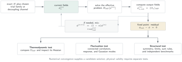
Mean-field iteration produces a candidate fixed point. Numerical convergence of the field residual is distinct from thermodynamic stability and from control of the fluctuations discarded by the approximation.

A practical iteration often uses mixing:

$$\boldsymbol\phi^{(n+1)} = (1-\alpha) \boldsymbol\phi^{(n)} + \alpha \mathcal F \left( \boldsymbol\phi^{(n)} \right),$$

with $0<\alpha\le1$ for simple under-relaxation. More advanced solvers use Anderson mixing, quasi-Newton updates, continuation, or direct minimization of a thermodynamic functional.

Convergence should be tested using more than the field increment. Useful residuals include

$$r_a = \mathcal F_a(\boldsymbol\phi) - \phi_a,$$

changes in the thermodynamic potential, symmetry constraints, particle-number constraints, and the stationarity gradient of the underlying functional.

Numerical Convergence Is Not Physical Stability

Linearize the fixed-point map around a solution $\boldsymbol\phi_*$:

$$\delta\boldsymbol\phi^{(n+1)} \simeq J_{\mathcal F} \delta\boldsymbol\phi^{(n)},$$

where

$$(J_{\mathcal F})_{ab} = \left. \frac{\partial\mathcal F_a} {\partial\phi_b} \right|_{\boldsymbol\phi_*}.$$

Plain iteration converges locally when the spectral radius obeys

$$\rho(J_{\mathcal F})<1.$$

Mixing changes the iteration Jacobian to

$$J_{\mathrm{mix}} = (1-\alpha)I + \alpha J_{\mathcal F}.$$

This is a statement about an algorithm. A physically stable equilibrium instead requires the appropriate energy or thermodynamic potential to be locally minimal with respect to admissible variations. A solver can be engineered to converge to a saddle, and a physically stable solution can be difficult for naive iteration.

Always separate:

1. small numerical residual;
2. local thermodynamic stability;
3. global comparison with other self-consistent solutions;
4. validity of the mean-field approximation itself.

Variational Structure at Zero Temperature

Let $\mathcal M$ be a normalized trial manifold. The restricted energy functional is

$$E_{\mathcal M} = \min_{ |\Psi\rangle\in\mathcal M } \langle\Psi|H|\Psi\rangle.$$

For admissible states and a Hamiltonian bounded below,

$$E_{\mathcal M} \ge E_0.$$

A product-state, Slater-determinant, coherent-state, or Gaussian mean field can therefore provide a rigorous upper bound to the ground-state energy when the expectation of the original Hamiltonian is evaluated exactly within the trial state.

The bound does not imply that:

• the state has high fidelity;
• an excitation gap is an upper or lower bound;
• a correlation function has a controlled sign of error;
• a broken-symmetry finite-size state is in the desired exact sector;
• a separately decoupled Hamiltonian retains the same variational guarantee.

Stationarity within a restricted manifold means only that the residual is orthogonal to represented tangent directions. Missing correlation directions can remain large.

Variational Structure at Finite Temperature

For a normalized density operator $\rho$, define

$$\mathcal F[\rho] = \operatorname{Tr}(\rho H) + k_{\mathrm B}T \operatorname{Tr}(\rho\ln\rho).$$

The exact Gibbs state minimizes this functional, and the minimum is the exact Helmholtz free energy:

$$F = \min_\rho \mathcal F[\rho].$$

Restricting $\rho$ to product or Gaussian density operators gives a variational mean-field free energy. Equivalently, for a solvable trial Hamiltonian $H_0$ with free energy $F_0$,

$$F \le F_0 + \langle H-H_0\rangle_0.$$

Optimizing the right-hand side over parameters in $H_0$ can generate self-consistency equations. This Gibbs–Bogoliubov–Feynman inequality is a free-energy upper bound, provided all quantities refer to the same Hamiltonian, ensemble, and temperature.

Order Parameters and Mean Fields

A mean field need not be an order parameter.

Order Parameters owns the general operator, symmetry, source, finite-size, and local-versus-nonlocal dictionary. This section explains how those variables enter a mean-field approximation.

Mean field	Typical operator	Symmetry role
density	$\langle n_i\rangle$	often symmetry preserving
magnetization	$\langle S_i^\alpha\rangle$	may break spin or time-reversal symmetry
condensate amplitude	$\langle b_i\rangle$	phase-referenced $U(1)$ breaking coordinate
pairing amplitude	$\langle c_i c_j\rangle$	anomalous $U(1)$ breaking coordinate
bond field	$\langle c_i^\dagger c_j\rangle$	may preserve or break translation and point-group symmetry
density wave	$\langle n_i\rangle-\bar n$	breaks translation symmetry
sublattice magnetization	$(-1)^i\langle S_i^z\rangle$	detects antiferromagnetic order

An order parameter transforms nontrivially under a symmetry and distinguishes phases or symmetry-related solutions. A Hartree density can be nonzero in every phase and simply parametrizes an inhomogeneous background.

Channel choice is physical input

The same interaction can be decoupled in density, magnetic, exchange, pairing, or bond channels. A chosen channel restricts which correlations can become self-consistent. If a calculation permits only uniform magnetization, it cannot discover a density wave, spiral, pair-density wave, or larger-unit-cell order.

An unbiased claim therefore requires either:

• a symmetry-complete set of plausible channels;
• a reason other channels are forbidden or parametrically suppressed;
• or an explicit statement that the calculation tests only a selected ansatz.

Algebraic rearrangements of an exact interaction can be equivalent before approximation but inequivalent after different terms are factorized. This is sometimes called a channel or Fierz ambiguity.

Symmetry Breaking Requires a Limit

A mean-field equation can possess nonzero order-parameter solutions even when a finite exact Hamiltonian has a unique symmetric ground state. This is useful, but its meaning must be stated carefully.

For a source $h$ coupled to an order parameter $M$, the many-body broken-symmetry value is characterized by an order such as

$$\lim_{h\to0^+} \lim_{V\to\infty} \langle M\rangle_h.$$

Mean field often works directly with one selected branch and thereby anticipates this limiting state. It does not prove that the finite system literally violates the exact symmetry.

Different mean-field solutions related by an exact symmetry have the same thermodynamic potential when the source vanishes. An optimizer’s preference for one branch can come from initialization, rounding, boundary conditions, or a deliberately applied seed.

For particle-number symmetry, a condensate or BCS state with a definite phase can organize local observables efficiently. The underlying finite-number Hamiltonian may still conserve $N$ exactly. Symmetry projection and number-conserving formulations can recover the exact sector while retaining the same leading bulk physics in an overlap regime.

Thermodynamic Potentials and Double Counting

Suppose an effective Hamiltonian depends on fields $\boldsymbol\phi$. Its quasiparticle or one-site eigenvalues alone are not generally the total mean-field energy. Constant terms from factorization must be included.

At finite temperature, define

$$\Omega_{\mathrm{MF}}(\boldsymbol\phi) = -\frac{1}{\beta} \ln \operatorname{Tr} e^{-\beta K_{\mathrm{MF}}(\boldsymbol\phi)}.$$

Here $K_{\mathrm{MF}}$ must contain every field-dependent subtraction term. Self-consistency often follows from

$$\frac{\partial\Omega_{\mathrm{MF}}} {\partial\phi_a} = 0.$$

When several stationary points exist, compare $\Omega_{\mathrm{MF}}$ in the same ensemble. Comparing a fixed-$N$ energy with a fixed-$\mu$ grand potential, or omitting a constant from only one phase, can reverse the apparent phase ordering.

The Hessian

$$\mathcal H_{ab} = \frac{\partial^2\Omega_{\mathrm{MF}}} {\partial\phi_a\partial\phi_b}$$

tests local stability within the represented field space. Positive eigenvalues indicate a local minimum under those variations; a zero eigenvalue can mark a continuous instability, a symmetry direction, or a redundant coordinate.

Linear Response and the Instability Criterion

Consider a scalar order parameter $m$ responding to an effective field

$$h_{\mathrm{eff}} = h+J_0m.$$

If the uncoupled building block has response

$$m \simeq \chi_0 h_{\mathrm{eff}},$$

then

$$m = \chi_0(h+J_0m).$$

The mean-field susceptibility is

$$\chi_{\mathrm{MF}} = \frac{\partial m}{\partial h} = \frac{\chi_0} {1-J_0\chi_0}.$$

The symmetric solution becomes linearly unstable when

$$1-J_0\chi_0 = 0.$$

This structure appears in magnetism, density waves, pairing, and other channels. The sign and matrix ordering depend on conventions, and a divergence of the approximate susceptibility diagnoses instability of the reference state rather than proving the exact phase on its own.

Worked Example: Classical Ising Ferromagnet

Consider spins $s_i=\pm1$ on a regular lattice of coordination number $z$:

$$H = -J \sum_{\langle ij\rangle} s_i s_j - h\sum_i s_i, \qquad J>0.$$

Each bond is counted once. Assume a uniform magnetization

$$m = \langle s_i\rangle.$$

Write

$$\begin{aligned} s_i s_j ={}& m(s_i+s_j) - m^2 \\ & + (s_i-m)(s_j-m). \end{aligned}$$

Discarding the final fluctuation product and using $Nz/2$ bonds gives

$$\begin{aligned} H_{\mathrm{MF}}(m) ={}& -(zJm+h) \sum_i s_i \\ & + \frac{NzJ}{2}m^2. \end{aligned}$$

Every spin is now independent in the self-consistent molecular field

$$h_{\mathrm{eff}} = h+zJm.$$

Partition function and free energy

The mean-field partition function is

$$\begin{aligned} Z_{\mathrm{MF}}(m) ={}& e^{-\beta NzJm^2/2} \\ &\times \Bigl[ 2\cosh \bigl( \beta(zJm+h) \bigr) \Bigr]^N. \end{aligned}$$

The free energy per site is therefore

$$\begin{aligned} f_{\mathrm{MF}}(m) ={}& \frac{zJ}{2}m^2 \\ & - \frac{1}{\beta} \ln\!\Bigl[ 2\cosh \bigl( \beta(zJm+h) \bigr) \Bigr]. \end{aligned}$$

Stationarity gives

$$\begin{aligned} 0 &= \frac{1}{zJ} \frac{\partial f_{\mathrm{MF}}}{\partial m} \\ &= m - \tanh \bigl( \beta(zJm+h) \bigr). \end{aligned}$$

Thus the self-consistency equation is

$$m = \tanh \bigl( \beta(zJm+h) \bigr).$$

Critical temperature

At $h=0$ and small $m$,

$$\begin{aligned} \tanh(\beta zJm) ={}& \beta zJm - \frac{(\beta zJm)^3}{3} \\ & + O(m^5). \end{aligned}$$

The symmetric solution loses stability when

$$\beta_c zJ = 1,$$

so

$$k_{\mathrm B}T_c^{\mathrm{MF}} = zJ.$$

For $T<T_c^{\mathrm{MF}}$, two symmetry-related nonzero solutions appear at zero field.

Landau expansion and critical exponent

Expanding the free energy at $h=0$ gives

$$\begin{aligned} f_{\mathrm{MF}}(m) ={}& f_0 + \frac{zJ}{2} (1-\beta zJ)m^2 \\ &+ \frac{\beta^3(zJ)^4}{12} m^4 + O(m^6). \end{aligned}$$

Close below $T_c^{\mathrm{MF}}$,

$$m^2 \simeq 3 \frac{T_c^{\mathrm{MF}}-T} {T_c^{\mathrm{MF}}}.$$

Hence

$$m \propto (T_c^{\mathrm{MF}}-T)^{1/2}.$$

The mean-field order-parameter critical exponent is $1/2$. It is not the exact exponent for short-range Ising systems below the upper critical dimension.

Susceptibility above the transition

Differentiate the self-consistency equation with respect to $h$. In the symmetric phase,

$$\chi = \frac{\partial m}{\partial h} = \beta(zJ\chi+1),$$

and therefore

$$\chi_{\mathrm{MF}} = \frac{\beta} {1-\beta zJ} = \frac{1} {k_{\mathrm B}(T-T_c^{\mathrm{MF}})}.$$

This is the Curie–Weiss divergence in the normalization used here.

What the Ising Example Gets Right and Wrong

The calculation correctly illustrates:

• a self-consistent molecular field;
• entropy competing with interaction energy;
• symmetric and symmetry-broken stationary points;
• susceptibility as a stability diagnostic;
• a continuous bifurcation in a scalar order parameter;
• an exactly solvable effective one-site problem.

It is quantitatively or qualitatively wrong when neglected spatial fluctuations dominate. The nearest-neighbor one-dimensional Ising model has no nonzero-temperature phase transition, while the mean-field equation predicts $k_{\mathrm B}T_c=2J$ because $z=2$. In two and three dimensions, mean field predicts the wrong short-range critical exponents and shifted transition temperatures. Critical Exponents and Scaling derives the mean-field exponent benchmark and explains its upper-critical-dimension and hyperscaling limits.

For an infinite-range Curie–Weiss model with properly scaled coupling, the magnetization becomes sharply concentrated in the thermodynamic limit away from critical singularities, and the same saddle-point equation becomes asymptotically exact for the bulk free energy.

Quantum Spin Mean Field

For the transverse-field Ising Hamiltonian

$$H = -J \sum_{\langle ij\rangle} \sigma_i^z\sigma_j^z - \Gamma \sum_i\sigma_i^x,$$

take

$$m = \langle\sigma_i^z\rangle.$$

The one-site mean-field Hamiltonian is

$$h_{\mathrm{MF}} = -zJm\,\sigma^z - \Gamma\sigma^x + \frac{zJ}{2}m^2.$$

Define

$$E(m) = \sqrt{ (zJm)^2 + \Gamma^2 }.$$

The finite-temperature self-consistency equation is

$$m = \frac{zJm}{E(m)} \tanh\bigl(\beta E(m)\bigr).$$

At zero temperature, a nonzero solution exists in this approximation when

$$\Gamma<zJ.$$

Thus

$$\Gamma_c^{\mathrm{MF}} = zJ.$$

The Transverse-Field Ising Model owns the exact one-dimensional solution and its actual critical convention. The comparison makes the mean-field limitation concrete: solving the local quantum problem exactly does not restore the spatial entanglement discarded by site factorization.

Common Mean-Field Families

Hartree

A product state replaces the interaction experienced by one particle with a potential generated by the average density of the others. The orbitals and density are solved self-consistently. Exchange and connected correlation are absent unless added by a richer ansatz.

Hartree–Fock

A Slater determinant enforces fermionic antisymmetry. Variation produces direct and exchange fields but omits correlation beyond a single determinant. Exchange is exact within that trial class; the exact many-body state generally is not a determinant.

Gross–Pitaevskii

A macroscopically occupied bosonic mode is represented by a complex field. Variation of the dilute-gas energy functional produces a nonlinear one-body equation. Control depends on diluteness and small depletion, not merely large particle number.

Lattice Gutzwiller mean field

A product of local states retains onsite number fluctuations exactly within each factor while factorizing intersite correlations. The Bose–Hubbard Model develops the resulting Mott-lobe approximation.

BCS mean field

An anomalous pairing field

$$\Delta \sim \langle c_{-\mathbf k\downarrow} c_{\mathbf k\uparrow} \rangle$$

turns a quartic pair-scattering interaction into a quadratic Bogoliubov Hamiltonian. The unprojected solution selects a phase and is not an eigenstate of microscopic particle number, although the exact reduced pairing Hamiltonian conserves number.

BCS Mean-Field Theory derives the Cooper logarithm, gap and number equations, coherence factors, thermodynamic potential, and symmetry caveats.

Hubbard magnetic mean field

For the onsite interaction

$$U n_{i\uparrow}n_{i\downarrow},$$

a density-channel decoupling gives

$$\begin{aligned} n_{i\uparrow}n_{i\downarrow} \longrightarrow{}& \langle n_{i\uparrow}\rangle n_{i\downarrow} + n_{i\uparrow} \langle n_{i\downarrow}\rangle \\ &- \langle n_{i\uparrow}\rangle \langle n_{i\downarrow}\rangle. \end{aligned}$$

Allowing spin- and site-dependent densities can represent ferro-, antiferro-, or density-wave patterns. Restricting the unit cell or omitting exchange and pairing channels restricts the answer before the equations are solved.

Mean Field and Gaussian Fluctuations

Mean field is often the first term in a hierarchy rather than the final theory. After finding a stationary configuration, restore small fluctuations:

$$O_a = \phi_a + \delta O_a.$$

Keeping terms quadratic in $\delta O_a$ produces a Gaussian theory. Depending on the system, this leads to:

• spin-wave theory around magnetic order;
• Bogoliubov modes around a condensate;
• random-phase response around a density or magnetic mean field;
• amplitude and phase modes around a pairing saddle;
• one-loop corrections to a thermodynamic potential.

The fluctuation spectrum also tests stability. A negative quadratic mode signals that the candidate saddle is unstable in a direction not stabilized by the current solution. A zero mode can be required by a continuous broken symmetry, but only if the approximation respects the associated conservation identities.

When Mean Field Can Be Controlled

Mean field is not controlled by “many particles” alone. Useful control can arise from specific structures.

Infinite-range or collective coupling

With interactions scaled so the energy is extensive, collective fields can obey a law of large numbers and their relative fluctuations can vanish as the system grows.

Large coordination

If each site couples weakly to many neighbors, individual neighbor fluctuations can average out. A standard large-$z$ limit scales a bond coupling as $J/z$ so that the total local field remains finite.

Large component number

In large-N or large-flavor theories, the effective action can scale as $N$, making saddle-point fluctuations parametrically small. The physical finite-$N$ correction must still be checked.

Dilute weakly interacting condensates

For a three-dimensional Bose gas, the gas parameter $na_s^3\ll1$ controls depletion and beyond-mean-field corrections. Macroscopic occupation helps identify the field, while diluteness supplies the actual small parameter.

High dimension or distance from criticality

Short-range fluctuations become less important in sufficiently high dimension. Even where mean field is qualitatively useful, it generally fails inside a fluctuation-dominated critical region whose size is estimated in Landau–Ginzburg Theory Preview by the Ginzburg criterion.

Restricted observables

Energy density or a coarse order parameter may be accurate while entanglement, spectral linewidths, or short-distance correlations are not. Control must be stated observable by observable.

Why Critical Regions Are Dangerous

Near a continuous transition, the correlation length grows and fluctuations become coherent over large regions. The assumption that each degree of freedom sees a narrowly distributed average environment then becomes least reliable.

Landau Theory owns the uniform analytic potential and the resulting mean-field exponent derivation. Below the upper critical dimension, long-wavelength fluctuations generally renormalize those exponents. At the upper critical dimension, logarithmic corrections can survive. Universality explains how dimension and order-parameter structure determine when a short-range critical point shares the mean-field fingerprint.

For short-range systems with a continuous symmetry, infrared fluctuations can forbid finite-temperature long-range order in low dimension under the hypotheses of the Hohenberg–Mermin–Wagner results. A static mean field can nevertheless produce a nonzero order parameter because it suppresses precisely those long-wavelength fluctuations.

This is not a small numerical error. It is a qualitative failure of the approximation’s fluctuation content.

Failure Modes Beyond Criticality

Mean field can also fail far from a conventional critical point.

Strong local correlations

A product or determinant state can misrepresent double occupancy, local moments, Mott localization, and multiplet structure even when no symmetry changes.

Low-dimensional entanglement

One-dimensional ground states can possess strong quantum correlations that no site-product state captures. A correct local expectation does not certify the correlation length or excitation spectrum.

Frustration and competing orders

Many nearly degenerate patterns can create a rugged free-energy landscape. A small unit cell or single-channel ansatz can select an artificial order.

Topological and fractionalized phases

Conventional local order parameters can miss long-range entanglement, gauge constraints, and fractional excitations. Parton mean fields may still be useful, but gauge fluctuations and projection are then central rather than optional details.

First-order transitions and metastability

Multiple local minima produce hysteresis and initialization dependence. A spinodal where one minimum disappears is not the same as the coexistence point where free energies cross.

Conservation-law violations

An inconsistent truncation can violate particle number, gauge covariance, Ward identities, or sum rules. A self-consistent approximation is not automatically conserving.

Dynamics

Static self-consistency does not supply collision integrals, damping, thermalization, or memory. Time-dependent mean-field equations can capture coherent collective motion but often miss scattering-induced relaxation.

Validation Checklist

Model and channel

• State the exact Hamiltonian, ensemble, and pair-counting convention.
• Name every retained field and its operator definition.
• State which competing channels, unit cells, and symmetries were allowed.
• Retain all constant and double-counting terms.

Solver

• Report field and stationarity residuals.
• Use several initial conditions and continuation directions.
• Distinguish numerical mixing stability from physical stability.
• Check particle-number, density, and other constraints independently.

Thermodynamics

• Compare all solutions using the same potential and ensemble.
• Inspect the Hessian or fluctuation kernel.
• Separate coexistence, spinodal, and continuous-instability points.
• Differentiate the full stationary potential, including implicit fields correctly.

Physics

• Recover exactly solvable and noninteracting limits.
• Estimate connected fluctuations or the first correction beyond mean field.
• Test sum rules, conservation laws, and symmetry relations.
• Compare with finite-size numerics or experiment in an overlap regime.
• State the dimension, interaction range, and distance from criticality.

Common Mistakes

• Writing a mean-field decoupling with an equals sign and no residual term.
• Omitting constant subtraction terms because they do not change eigenvectors.
• Treating self-consistency as an accuracy estimate.
• Calling every mean field an order parameter.
• Restricting to one channel and claiming no competing order exists.
• Comparing stationary solutions in different ensembles.
• Selecting the solution reached by iteration without comparing thermodynamic potentials.
• Confusing convergence of the iterative map with a positive thermodynamic Hessian.
• Reporting a spinodal as a phase boundary.
• Assuming a large particle count makes mean field exact.
• Applying a uniform ansatz to an antiferromagnet or density wave.
• Inferring exact finite-system symmetry breaking from a nonzero mean-field field.
• Treating an anomalous BCS average as proof that the exact Hamiltonian violates number conservation.
• Ignoring Mermin–Wagner or other low-dimensional infrared constraints.
• Using mean-field critical exponents inside a fluctuation-dominated region.
• Calling Hartree–Fock correlation energy “exchange” or vice versa.
• Projecting a saddle-point state without re-evaluating its energy and observables.
• Assuming a local minimum is the global equilibrium solution.
• Using static mean field to infer lifetimes or thermalization rates.
• Failing to transform observables consistently when the effective basis changes.

Exercises

The discarded connected fluctuation

Starting from $A=\langle A\rangle+\delta A$ and $B=\langle B\rangle+\delta B$, show that the error in the factorized expectation value is a connected correlator.

Solution

Taking the expectation of the exact decomposition gives

$$\langle AB\rangle = \langle A\rangle \langle B\rangle + \langle\delta A\,\delta B\rangle.$$

Therefore the factorization

$$\langle AB\rangle \approx \langle A\rangle \langle B\rangle$$

discards

$$\langle\delta A\,\delta B\rangle = \langle AB\rangle - \langle A\rangle \langle B\rangle,$$

which is the connected two-point correlation in this ordering. Self-consistency fixes the one-point functions but does not force this term to be small.

Bond counting in the Ising mean field

Derive the constant $NzJm^2/2$ in the uniform Ising mean-field Hamiltonian.

Solution

For each bond,

$$s_i s_j \longrightarrow m(s_i+s_j)-m^2.$$

The linear terms give $z$ copies of $m s_i$ at each site, so

$$-J \sum_{\langle ij\rangle} m(s_i+s_j) = -zJm\sum_i s_i.$$

There are $Nz/2$ bonds. The constant contribution is

$$-J \sum_{\langle ij\rangle} (-m^2) = \frac{NzJ}{2}m^2.$$

The factor $1/2$ is bond counting, not an adjustable convention.

Landau expansion and spontaneous magnetization

Use the expansion of $f_{\mathrm{MF}}(m)$ at $h=0$ to find the leading nonzero magnetization below $T_c^{\mathrm{MF}}$.

Solution

Write

$$f(m) = f_0+a_2m^2+a_4m^4+O(m^6),$$

with

$$a_2 = \frac{zJ}{2}(1-\beta zJ), \qquad a_4 = \frac{\beta^3(zJ)^4}{12}.$$

The nonzero stationary solution obeys

$$2a_2m+4a_4m^3=0,$$

so

$$m^2 = -\frac{a_2}{2a_4} = 3 \frac{ \beta zJ-1 }{ (\beta zJ)^3 }.$$

Near $T_c^{\mathrm{MF}}$, this becomes

$$m^2 \simeq 3 \frac{T_c^{\mathrm{MF}}-T} {T_c^{\mathrm{MF}}},$$

which yields the mean-field exponent $1/2$.

Curie–Weiss susceptibility

Differentiate

$$m = \tanh \bigl[ \beta(zJm+h) \bigr]$$

and derive the susceptibility for arbitrary self-consistent $m$.

Solution

Let $\chi=\partial m/\partial h$. Differentiation gives

$$\chi = \beta \operatorname{sech}^2 \bigl[ \beta(zJm+h) \bigr] (zJ\chi+1).$$

At a self-consistent solution,

$$\operatorname{sech}^2 \bigl[ \beta(zJm+h) \bigr] = 1-m^2.$$

Therefore

$$\chi = \frac{ \beta(1-m^2) }{ 1-\beta zJ(1-m^2) }.$$

For $m=0$, this reduces to $\beta/(1-\beta zJ)$.

Quantum Ising critical field

At zero temperature, solve the quantum-spin mean-field equation for the nonzero magnetization.

Solution

At $T=0$, $\tanh(\beta E)\to1$, so a nonzero $m$ obeys

$$1 = \frac{zJ} {\sqrt{(zJm)^2+\Gamma^2}}.$$

Hence

$$(zJm)^2 = (zJ)^2-\Gamma^2,$$

and

$$m = \pm \sqrt{ 1- \left( \frac{\Gamma}{zJ} \right)^2 }.$$

The nonzero solution exists for $\Gamma<zJ$ and vanishes continuously at $\Gamma_c^{\mathrm{MF}}=zJ$.

Why the subtraction constant matters

Suppose one incorrectly drops $zJm^2/2$ from the Ising free energy. Show that the correct self-consistency equation is no longer its stationarity condition.

Solution

The incorrect per-site expression would be

$$\begin{aligned} f_{\mathrm{bad}}(m) &= -\frac{1}{\beta} \ln \mathcal C(m), \\ \mathcal C(m) &:= 2\cosh \bigl( \beta(zJm+h) \bigr). \end{aligned}$$

Its derivative is

$$\frac{df_{\mathrm{bad}}}{dm} = -zJ \tanh \bigl( \beta(zJm+h) \bigr).$$

At a self-consistent point this equals $-zJm$, which vanishes only for $m=0$. The nonzero self-consistent states are therefore not stationary points of the incorrectly truncated free energy. Restoring $zJm^2/2$ adds $zJm$ to the derivative and repairs the variational structure.

Bipartite antiferromagnetic mean field

For

$$H = J \sum_{\langle ij\rangle} s_i s_j, \qquad J>0,$$

on a bipartite lattice, take $m_A=-m_B=m$ at zero field. Derive the self-consistency equation and transition temperature.

Solution

An $A$-sublattice spin sees $z$ neighbors with mean $m_B=-m$. Its effective energy is

$$Jz s_A m_B = -zJm s_A.$$

Thus

$$m_A = \tanh(\beta zJm).$$

The $B$ equation gives the opposite sign consistently. Therefore

$$m = \tanh(\beta zJm),$$

and the linear instability occurs at

$$k_{\mathrm B}T_N^{\mathrm{MF}} = zJ.$$

A uniform one-field ansatz would miss this ordered pattern, illustrating why the allowed unit cell is part of the approximation.

Mixing and local convergence

For a scalar fixed-point equation $\phi=\mathcal F(\phi)$, show how linear mixing changes the local convergence factor near $\phi_*$.

Solution

Let $\delta_n=\phi_n-\phi_*$. Linearizing gives

$$\mathcal F(\phi_n) - \phi_* \simeq \mathcal F'(\phi_*)\delta_n.$$

The mixed update produces

$$\delta_{n+1} \simeq \left[ 1-\alpha + \alpha\mathcal F'(\phi_*) \right] \delta_n.$$

The local numerical convergence condition is therefore

$$\left| 1-\alpha + \alpha\mathcal F'(\phi_*) \right| <1.$$

Changing $\alpha$ can stabilize the iteration without changing the underlying fixed point or its thermodynamic Hessian. Algorithmic and physical stability remain separate questions.

Key Takeaways

• Mean field replaces an interacting environment by self-consistent expectation-value fields.
• Factorization, restricted variation, and saddle-point approximation are complementary formulations, but arbitrary truncations need not be equivalent.
• The discarded object is a product of fluctuations, so self-consistency does not make correlation corrections vanish.
• Constant subtraction terms are required for correct energies and thermodynamic potentials.
• A converged fixed point must still be tested for local and global thermodynamic stability.
• A mean field can be a density or constraint field without being an order parameter.
• Broken-symmetry mean-field states represent selected bulk branches; they do not prove finite-system symmetry breaking.
• Mean field can be controlled by infinite range, large coordination, large component number, diluteness, or another explicit parameter.
• Critical, low-dimensional, frustrated, topological, and strongly correlated regimes often require fluctuations or a richer ansatz.
• Method validity is observable-dependent and should be checked against limits, sum rules, corrections, and independent benchmarks.

Cross-Links

• Interacting Many-Body Systems Overview
• Two-Body Operators
• Variational Principle
• Thermodynamic Limit
• Spontaneous Symmetry Breaking Preview
• Fluctuations and Susceptibilities
• Correlation Functions Overview
• Quantum Phase Transitions
• Hubbard Model
• Stoner Criterion — a material-facing stability calculation that separates quadratic spinodal, nonlinear minimum, and fluctuation limitations.
• Bose–Hubbard Model
• Weakly Interacting Bose Gas Preview
• BCS Mean-Field Theory
• BCS Model
• Common Many-Body Hamiltonians
• Choosing an Approximation Method

References

• P. Weiss, “L’hypothèse du champ moléculaire et la propriété ferromagnétique,” Journal de Physique Théorique et Appliquée 6, 661–690 (1907), doi:10.1051/jphystap:019070060066100.
• W. L. Bragg and E. J. Williams, “The Effect of Thermal Agitation on Atomic Arrangement in Alloys,” Proceedings of the Royal Society A 145, 699–730 (1934), doi:10.1098/rspa.1934.0132.
• J. Hubbard, “Electron Correlations in Narrow Energy Bands,” Proceedings of the Royal Society A 276, 238–257 (1963), doi:10.1098/rspa.1963.0204.
• J. Bardeen, L. N. Cooper, and J. R. Schrieffer, “Theory of Superconductivity,” Physical Review 108, 1175–1204 (1957), doi:10.1103/PhysRev.108.1175.
• N. D. Mermin and H. Wagner, “Absence of Ferromagnetism or Antiferromagnetism in One- or Two-Dimensional Isotropic Heisenberg Models,” Physical Review Letters 17, 1133–1136 (1966), doi:10.1103/PhysRevLett.17.1133.
• P. C. Hohenberg, “Existence of Long-Range Order in One and Two Dimensions,” Physical Review 158, 383–386 (1967), doi:10.1103/PhysRev.158.383.
• A. L. Fetter and J. D. Walecka, Quantum Theory of Many-Particle Systems, Dover (2003).
• J. W. Negele and H. Orland, Quantum Many-Particle Systems, Westview Press (1998).
• N. Goldenfeld, Lectures on Phase Transitions and the Renormalization Group, CRC Press (2018), doi:10.1201/9780429493492.
• P. M. Chaikin and T. C. Lubensky, Principles of Condensed Matter Physics, Cambridge University Press (1995), doi:10.1017/CBO9780511813467.
• S. Sachdev, Quantum Phase Transitions, 2nd ed., Cambridge University Press (2011), doi:10.1017/CBO9780511973765.
• P. Coleman, Introduction to Many-Body Physics, Cambridge University Press (2015), doi:10.1017/CBO9781139020916.