Diagrammatic Methods Preview

A many-body diagram is a compact representation of one algebraic term or one class of terms in an expansion of a correlation function, energy, free energy, response, or effective interaction. Lines encode specified two-point functions or interactions. Vertices encode specified couplings. Topology organizes contractions, signs, conservation laws, and repeated structures.

A diagram is not:

• a literal trajectory followed by a microscopic particle;
• a complete physical process independent of its mathematical rules;
• an approximation merely because it has been drawn;
• uniquely defined without an ordering convention, reference state, and observable;
• interchangeable across real time, imaginary time, stationary perturbation theory, and QFT.

The basic chain is

$$\text{ordered operator expansion} \longrightarrow \text{Wick contractions} \longrightarrow \text{algebraic terms} \longrightarrow \text{diagram topologies}.$$

The value lies in the last step: many long sums differ only by labels while sharing the same topology. Once the rules are fixed, diagrams expose which terms are connected, reducible, repeated, dominant, or required by symmetry.

Canonical Scope

This page is the canonical preview of:

• how a Gaussian reference and Wick’s theorem generate diagrams;
• reference propagators, interaction lines, external legs, and vertices;
• momentum, frequency, spin, and flavor routing;
• perturbative order and internal sums;
• the closed-fermion-loop sign and exchange signs;
• connected, disconnected, amputated, one-particle-irreducible, and skeleton topologies;
• self-energy and the Dyson equation;
• particle–hole bubbles and their relation to polarization;
• the distinction among Goldstone, Matsubara, real-time, and QFT diagrams;
• dressed-line double counting;
• elementary self-energy–vertex consistency and Ward-identity motivation;
• ultraviolet, infrared, and analytic-continuation caveats;
• when the subject has crossed into full QFT or specialized many-body field theory.

Neighboring pages retain separate ownership:

• Wick’s Theorem Preview owns normal ordering plus contractions as operator algebra.
• Perturbation Theory in Many-Body Systems owns reference states, particle–hole intermediate sectors, linked-cluster volume counting, and infrared failure of fixed-order expansions.
• Normal Ordering in Many-Body QM owns exact reference-state Hamiltonian decomposition.
• Random Phase Approximation owns the bubble-chain approximation, screening, dielectric response, and collective poles.
• Hartree–Fock Approximation owns the variational direct and exchange fields.
• Finite-Temperature QM Overview owns the common Gibbs-operator, thermal-circle, KMS, Matsubara, spectral, and path-integral map.
• Matsubara Formalism Preview owns the compact-time Fourier workflow, loop-sum measure, convergence prescriptions, and zero-temperature limit.
• Bosonic and Fermionic Matsubara Frequencies owns the graded grids, units, index arithmetic, parity assignments, and finite cutoffs used in routing.
• Thermal Green Functions owns the ordered propagator definitions, equal-time contacts, occupations, and free thermal lines.
• Green Functions in Many-Body QM owns addition and removal Lehmann representations, poles, spectral weights, quasiparticle meaning, and the canonical comparison of retarded and Matsubara Green functions.
• Spectral Functions owns how a continued self-energy becomes a line shape, residue, linewidth, and experimentally convolved signal.
• What Is a Green Function? and From Green Functions in QM to QFT own the one-particle mathematical and QFT-facing bridges.
• From Sources in QM to Generating Functionals in QFT owns the source-functional route to field-theory diagrams.

This page teaches enough grammar to read an elementary many-body diagram and reconstruct its formula. It does not develop renormalized perturbation theory, LSZ reduction, gauge fixing, non-Abelian diagrammatics, full Bethe–Salpeter or parquet equations, Schwinger–Keldysh contours, or production diagrammatic Monte Carlo. Those require the corresponding specialized or QFT treatment.

Fix the Convention Before Drawing

The same topology can represent different formulas in different conventions. Before using a diagram, state:

1. the Hamiltonian or action;
2. the reference state or ensemble;
3. real time, imaginary time, stationary energy denominators, or a contour;
4. bosonic or fermionic statistics;
5. normal-ordering and contraction convention;
6. Fourier-transform normalization;
7. whether lines are bare, mean-field, partially dressed, or fully dressed;
8. whether the interaction is bare, screened, antisymmetrized, or mediated by another field;
9. the definition and sign of every Green function and response function;
10. the regulator and external kinematics.

Line style is not universal. A dashed line can mean a bare interaction in one text, a phonon in another, or an auxiliary field in a third. The legend is part of the calculation.

Working Matsubara convention

For a concrete grammar, use a normal-state fermionic reference at temperature $T$. Define

$$G_0(1,2) = -\left\langle \mathcal T_\tau \psi(1) \psi^\dagger(2) \right\rangle_0.$$

For a translation-invariant diagonal reference,

$$G_0(\mathbf k,i\omega_n) = \frac{1}{ i\omega_n-\xi_{\mathbf k} },$$

where

$$\omega_n = (2n+1)\pi T$$

is a fermionic Matsubara frequency and

$$\xi_{\mathbf k} = \epsilon_{\mathbf k}-\mu.$$

This formula defines the solid directed line used below. It is a reference propagator, not yet a statement about the exact interacting spectrum.

Instantaneous density interaction

Take a two-body interaction

$$\begin{aligned} V &= \frac{1}{2\mathcal V} \sum_{\mathbf k,\mathbf k',\mathbf q} \sum_{\sigma,\sigma'} v_{\mathbf q} \\ &\quad\times c_{\mathbf k+\mathbf q,\sigma}^\dagger c_{\mathbf k'-\mathbf q,\sigma'}^\dagger c_{\mathbf k',\sigma'} c_{\mathbf k,\sigma}. \end{aligned}$$

One may represent $v_{\mathbf q}$ by a dashed interaction line joining two density vertices. Alternatively, one may use one antisymmetrized four-fermion vertex. These are different bookkeeping conventions; exchange must not be built into the vertex and then added again as a separate exchange graph.

From the Ordered Expansion to Diagrams

For an imaginary-time observable $O$,

$$\langle O\rangle = \frac{ \left\langle \mathcal T_\tau O_I \exp\!\left[ -\lambda \int_0^\beta d\tau\, V_I(\tau) \right] \right\rangle_0 }{ \left\langle \mathcal T_\tau \exp\!\left[ -\lambda \int_0^\beta d\tau\, V_I(\tau) \right] \right\rangle_0 }.$$

Expanding the numerator gives

$$\begin{aligned} \langle O\rangle_{\mathrm{num}} &= \sum_{n=0}^{\infty} \frac{(-\lambda)^n}{n!} \\ &\quad\times \int_0^\beta d\tau_1\cdots d\tau_n \left\langle \mathcal T_\tau O_I V_I(\tau_1)\cdots V_I(\tau_n) \right\rangle_0. \end{aligned}$$

If the reference is Gaussian, Wick’s theorem rewrites each ordered expectation value as a sum over complete contraction patterns. Every contraction contributes a reference two-point function. Every insertion of $V$ contributes a vertex. A diagram records the connectivity of one contraction pattern after equivalent labelings are grouped.

Why the denominator is present

The denominator contains diagrams with no connection to the external operator $O$. These vacuum pieces multiply every numerator contribution. Dividing removes them.

Equivalently, the logarithm of a partition or projection amplitude retains connected vacuum diagrams. Vacuum normalization and connectedness are related but distinct operations:

• the denominator removes vacuum factors from normalized correlators;
• selecting connected diagrams removes pieces disconnected from the external insertions;
• taking a logarithm selects connected vacuum contributions to free energies.

The factorial and symmetry factors

The factor $1/n!$ compensates permutations of $n$ identical interaction insertions. Many permutations generate the same labeled contraction topology and cancel part or all of this factorial. A residual symmetry factor remains when a diagram has automorphisms that leave it unchanged.

One cannot assign a symmetry factor from the picture alone unless the vertex normalization, line types, and whether labels are distinguishable have been specified.

The Elementary Dictionary

For the working convention:

Graphical object	Algebraic meaning
directed solid internal line	$G_0(\mathbf k,i\omega_n)$ or a declared dressed $G$
dashed interaction line	$v_{\mathbf q}$, including its normalization and sign convention
interaction vertex	coupling factor plus momentum, frequency, spin, and flavor conservation
external solid leg	field insertion defining a one-particle correlator
external source leg	density, spin, current, or other operator insertion
closed fermion loop	internal momentum-frequency sum and one extra factor $-1$
repeated identical topology	symmetry or combinatorial factor

An internal fermion line contributes

$$T \sum_{\omega_n} \int_{\mathbf k} G_0(\mathbf k,i\omega_n),$$

only as part of the complete product dictated by the graph. Here

$$\int_{\mathbf k} \equiv \int_{\mathrm{BZ}} \frac{d^d k}{(2\pi)^d}$$

for a lattice Brillouin zone, or a regulated continuum integral.

Conservation at a vertex

At an instantaneous two-body vertex,

$$\mathbf k_1+\mathbf k_2 = \mathbf k_3+\mathbf k_4$$

and

$$\omega_1+\omega_2 = \omega_3+\omega_4.$$

Spin or flavor is conserved or transformed according to the interaction tensor. Drawing an unlabeled vertex does not remove these Kronecker or Dirac delta functions; it suppresses them visually.

Arrows

For a number-conserving fermion propagator, an arrow records the orientation of fermionic contraction and conserved charge flow. In a hole interpretation, the same line segment can be read relative to a filled reference. In Nambu notation, line and arrow conventions change because normal and anomalous propagators are combined.

An arrow is not a classical path through space.

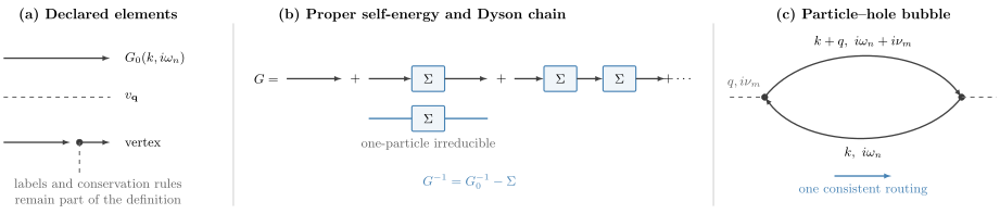
A solid directed line denotes a declared propagator, and a dashed line denotes a declared interaction. A proper self-energy insertion $\Sigma$ repeats through Dyson’s equation. A closed two-line particle–hole loop defines a polarization bubble, with momentum and frequency routed consistently through both lines.

Perturbative Order and Power Counting

If every interaction insertion carries $\lambda$, a diagram with $V_d$ interaction vertices is nominally order

$$\lambda^{V_d}.$$

That statement is only the first layer. The actual size also depends on:

• powers of volume from loop sums and line normalization;
• spin, flavor, or component sums;
• energy denominators or low-frequency propagators;
• small external momentum or frequency;
• long-range interaction kernels;
• occupation factors and Fermi-surface geometry;
• symmetry factors and cancellations;
• logarithms generated by broad scale intervals.

A high-order diagram can dominate a lower-order one in an infrared-enhanced channel. Conversely, a nominally allowed diagram can vanish by symmetry, kinematics, or antisymmetry.

Large-N counting

If a closed matter loop sums over $N$ flavors, it can contribute a factor $N$. A vertex may carry $1/N$. Counting loops and vertices then organizes diagrams by powers of $1/N$.

Large-N and Saddle-Point Methods Preview owns the model scaling and fluctuation hierarchy. The diagram by itself does not reveal which $N$ is large.

Volume counting

Each independent internal momentum sum contributes a power of volume in finite normalization; each translation-invariant interaction matrix element carries compensating inverse powers. Connected vacuum or energy diagrams should combine to an extensive result when infrared and ultraviolet behavior is regular.

Disconnected products can carry higher powers of volume. Their cancellation belongs to the linked-cluster structure developed in Perturbation Theory in Many-Body Systems.

Fermionic Signs

Fermionic signs come from anticommuting operators into the order needed to form contractions.

Closed-loop sign

Each closed fermion loop contributes an additional factor

$$-1.$$

For example, the independent particle–hole bubble in the working convention is

$$\begin{aligned} \Pi_0( \mathbf q, i\nu_m ) &= -g T \sum_{\omega_n} \int_{\mathbf k} G_0( \mathbf k+\mathbf q, i\omega_n+i\nu_m ) \\ &\qquad\times G_0( \mathbf k, i\omega_n ), \end{aligned}$$

where $g$ is a spin or flavor degeneracy when all components have the same propagator.

The leading minus sign is the closed-fermion-loop sign in this definition of $\Pi_0$. Some texts define the susceptibility as $-\Pi$, absorb a minus sign into the vertex, or reverse Fourier conventions. Copying the formula without copying the definitions is unsafe.

Exchange sign

Interchanging two external or internal fermionic labels introduces an antisymmetry sign. One may handle exchange by:

• drawing direct and exchange contractions separately with their signs; or
• using antisymmetrized vertices that combine them.

Doing both double counts exchange.

Loop count is not the whole sign

The full sign can also depend on:

• the ordering of external fermionic operators;
• anomalous Nambu conventions;
• how an antisymmetrized matrix element is defined;
• permutation of identical external legs;
• contour-branch indices in nonequilibrium theory.

“Minus one per loop” is a rule within a complete convention, not a substitute for deriving that convention.

Connected, Reducible, and Skeleton Diagrams

Several topological classifications answer different questions.

Class	Definition	Typical role
disconnected	graph has more than one connected component	cancels from normalized connected correlators or exponentiates in $Z$
connected	every part is linked to every other part	contributes to connected correlators
one-particle reducible	cutting one internal single-particle line disconnects the graph	generated by repeated self-energy insertion
one-particle irreducible	cannot be disconnected by cutting one internal single-particle line	belongs to the proper self-energy or 1PI vertex
amputated	external propagator factors have been removed	isolates a proper vertex or scattering kernel
skeleton	built from dressed lines with no explicit self-energy insertion subgraph	used in self-consistent functionals

Connected does not imply one-particle irreducible. A chain of two proper self-energy insertions on one propagator is connected but one-particle reducible.

Two-particle reducibility is channel dependent

A four-point graph can be reducible by cutting two lines in:

• the direct particle–hole channel;
• the crossed particle–hole channel;
• the particle–particle channel.

The same graph can be irreducible in one channel and reducible in another. Bethe–Salpeter and parquet methods organize this channel dependence. Their full equations lie beyond this preview.

Self-Energy

The proper self-energy $\Sigma$ is the sum of one-particle-irreducible two-point insertions in a declared expansion.

The Dyson equation is

$$G = G_0 + G_0\Sigma G.$$

In a translation-invariant scalar notation,

$$G^{-1}( \mathbf k, i\omega_n ) = G_0^{-1}( \mathbf k, i\omega_n ) -\Sigma( \mathbf k, i\omega_n ).$$

Iterating once gives

$$\begin{aligned} G ={}& G_0 + G_0\Sigma G_0 + G_0\Sigma G_0\Sigma G_0 + \cdots. \end{aligned}$$

Thus $\Sigma$ is not merely an energy shift. It is the irreducible kernel whose repeated insertion dresses propagation.

Hartree and Fock contributions

For a two-body fermion interaction, first-order self-energy terms commonly include:

• a Hartree direct term determined by an average density;
• a Fock exchange term produced by antisymmetry.

For an instantaneous interaction and a stationary normal reference, these terms can be frequency independent. Hartree–Fock Approximation owns their variational derivation and physical interpretation.

Higher-order self-energies can depend on momentum and frequency. After a justified analytic continuation, their real and imaginary parts affect dispersion and damping. Green Functions in Many-Body QM owns the canonical pole and Lehmann interpretation. Spectral Functions owns how the resulting self-energy is converted into quasiparticle positions, residues, linewidths, and line shapes.

Reference subtraction

If $G_0$ already contains a Hartree–Fock potential, the perturbation must include a counterterm that subtracts it. Otherwise the first-order self-energy is counted once in $G_0$ and again as an insertion.

This is the diagrammatic form of the repartitioning rule:

$$H = \left( H_{\mathrm{free}}+U_{\mathrm{ref}} \right) + \left( H_{\mathrm{int}}-U_{\mathrm{ref}} \right).$$

Bubble Diagrams

A bubble is a closed loop made from two single-particle propagators joined by two operator or interaction vertices. In a density channel, it describes the independent propagation of a particle–hole pair between two density insertions.

The Matsubara sum gives

$$\begin{aligned} \Pi_0( \mathbf q, i\nu_m ) &= g \int_{\mathbf k} \frac{ n_{\mathrm F}( \xi_{\mathbf k+\mathbf q} ) -n_{\mathrm F}( \xi_{\mathbf k} ) }{ i\nu_m -\xi_{\mathbf k+\mathbf q} +\xi_{\mathbf k} }. \end{aligned}$$

This expression follows from the preceding sign convention. Algebraically equivalent forms can move a minus sign between numerator and denominator.

What one bubble contains

One bubble contains:

• Pauli occupation factors;
• the independent particle–hole continuum;
• momentum and energy transfer from the external source;
• spin or flavor multiplicity;
• the reference dispersion.

It does not by itself contain:

• screening to all orders;
• self-energy broadening;
• vertex corrections;
• multiple particle–hole pairs;
• a collective pole outside the independent continuum.

Bubble chains

The RPA page uses a density-response convention whose independent polarization is the negative of the loop function defined above:

$$\Pi_0^{(\mathrm{resp})} = -\Pi_0^{(\mathrm{loop})}.$$

This sign is part of the response definition and interaction-vertex convention; it is not an additional fermion-loop sign. In that response convention, joining bubbles by repeated density interactions produces

$$\Pi^{(\mathrm{resp})} = \Pi_0^{(\mathrm{resp})} + \Pi_0^{(\mathrm{resp})} v \Pi_0^{(\mathrm{resp})} + \Pi_0^{(\mathrm{resp})} v \Pi_0^{(\mathrm{resp})} v \Pi_0^{(\mathrm{resp})} + \cdots.$$

Therefore

$$\Pi_{\mathrm{RPA}}^{(\mathrm{resp})} = \frac{ \Pi_0^{(\mathrm{resp})} }{ 1-v\Pi_0^{(\mathrm{resp})} }.$$

Random Phase Approximation owns this resummation, its sign audit, screening, collective modes, and failure modes. This page owns only how the bubble topology translates into the two-propagator loop.

Not every two-line loop is the same channel

Pairing diagrams contain two fermion lines but organize particle–particle propagation rather than particle–hole propagation. Nambu bubbles can include anomalous propagators. A visual loop is not enough to identify the channel; arrows, external labels, and momentum routing matter.

Vertex Corrections

A vertex correction changes the coupling between an external source or interaction and the propagating particles. It can encode:

• exchange between a particle and a hole;
• repeated scattering in one channel;
• screening or local-field effects;
• coupling to collective modes;
• constraints required by a conservation law.

Let $\Gamma^\mu$ be the full vertex for a conserved $U(1)$ current. A Ward identity has the structural form

$$q_\mu \Gamma^\mu(k+q,k) = G^{-1}(k+q) -G^{-1}(k),$$

with components, factors of charge, $i$, and metric conventions fixed by the real- or imaginary-time formulation.

This relation says that self-energy and vertex corrections are not independent decorations. Changing $G$ changes the vertex structure required by charge conservation.

Bare bubble with dressed lines

Replacing $G_0$ by a dressed $G$ inside a bubble while keeping the bare density vertex can violate a Ward identity. It may be a useful approximation in a specified regime, but it is not automatically conserving.

The required correction depends on how the self-energy was generated. There is no universal vertex patch that repairs every dressed propagator.

Bare, Dressed, and Skeleton Expansions

Bare expansion

A bare expansion uses:

• fixed $G_0$ lines;
• fixed bare interactions;
• all diagrams through a declared order.

Its order counting is transparent, but a low-order truncation may poorly describe shifted poles or collective screening.

Dressed-line expansion

One may solve a Dyson equation and use $G$ in internal lines. This resums infinitely many bare self-energy insertions. If the original insertion diagrams are then retained explicitly, they are double counted.

Skeleton expansion

A skeleton expansion uses dressed propagators but retains only diagrams without explicit self-energy insertion subgraphs. The self-energy is obtained self-consistently from those skeletons.

This can improve consistency, but:

• self-consistency does not guarantee accuracy;
• multiple solutions can occur;
• vertex corrections must still be matched;
• nominal bare perturbative order is no longer the only ordering variable.

Functional consistency preview

In a conserving construction, one builds a functional $\Phi[G]$ from selected closed skeleton diagrams and defines

$$\Sigma = \frac{\delta\Phi}{\delta G}$$

up to convention-dependent signs and factors. Further derivatives generate compatible vertex kernels.

This Baym–Kadanoff or Luttinger–Ward logic explains why a coherent family of diagrams can preserve conservation laws better than an arbitrary list of individually plausible graphs. Its existence, uniqueness, and practical validity are nontrivial and belong to advanced many-body field theory.

Goldstone, Matsubara, and Real-Time Diagrams

Goldstone diagrams

Stationary many-body perturbation theory often uses Goldstone diagrams:

• time flows in one direction;
• particle and hole lines are defined relative to a reference determinant;
• intermediate states carry explicit energy denominators;
• each time ordering can be displayed separately.

They are natural for ground-state energies and wavefunction amplitudes.

Matsubara diagrams

Equilibrium finite-temperature diagrams use imaginary time:

• fermionic frequencies are $(2n+1)\pi T$;
• bosonic frequencies are $2m\pi T$;
• internal frequencies are summed;
• time orderings are combined into propagators;
• analytic continuation may later connect to real-frequency functions.

One Matsubara or Feynman graph can combine several Goldstone time orderings. Their numerical factors and denominators should not be transferred by visual analogy.

Real-time time-ordered diagrams

Zero-temperature time-ordered propagators use real frequencies with causal prescriptions. Retarded, advanced, lesser, greater, and time-ordered functions are distinct. A time-ordered self-energy cannot be inserted blindly into a retarded Dyson equation without the correct continuation or contour relation.

Nonequilibrium contours

Driven or transient systems often require a forward-and-backward time contour. Every line and vertex then carries a contour index or Keldysh component. Real-Time Thermal Dynamics Preview owns the initial-state and contour motivation; full Schwinger–Keldysh rules belong to QFT.org or a dedicated nonequilibrium many-body treatment.

Analytic Continuation

A Matsubara function is known initially at discrete imaginary frequencies. For a function with the required analyticity and spectral behavior, the retarded quantity is obtained by continuation

$$i\nu_m \longrightarrow \omega+i0^+.$$

Several cautions matter:

• perform internal Matsubara sums and derive the analytic function before substituting;
• preserve branch cuts and thresholds, not only poles;
• continue the complete conserving combination when cancellations matter;
• numerical continuation from noisy data is ill conditioned;
• a finite broadening $\eta$ is not automatically a physical lifetime.

Retarded and Advanced Green Functions owns causal boundary values in the one-particle setting. Green Functions in Many-Body QM owns the normal many-body retarded and Matsubara spectral bridge, including the ill-conditioned numerical-continuation warning.

Ultraviolet and Infrared Audits

Diagrams expose divergences; they do not remove them.

Ultraviolet

Continuum loops can diverge at large internal momentum or frequency. A calculation must state:

• regulator;
• bare parameters;
• matching or renormalization prescription;
• counterterms;
• which observable is cutoff independent.

Normal ordering can remove selected vacuum contractions but does not renormalize every local product.

Infrared

Gapless lines, Fermi surfaces, Goldstone modes, or long-range interactions can enhance low-energy regions. Look for:

$$\ln\!\left( \frac{\Lambda}{E} \right), \qquad E^{-\alpha}, \qquad \ln L, \qquad T^{-\gamma}.$$

If a family of diagrams has the same enhanced scaling at all orders, fixed-order truncation is not controlled. One must identify and resum the relevant channel.

External limits

For response functions,

$$\lim_{\omega\to0} \lim_{\mathbf q\to0}$$

can differ from

$$\lim_{\mathbf q\to0} \lim_{\omega\to0}.$$

The diagram formula does not choose the physical limit. The measurement or thermodynamic question does.

Reading a Diagram Reliably

Given a published graph:

1. find the legend and action;
2. identify external operators and their ordering;
3. determine whether every internal line is bare or dressed;
4. label all external momenta, frequencies, spins, and flavors;
5. choose independent loop variables;
6. impose conservation at each vertex;
7. multiply line and vertex factors;
8. include closed-fermion-loop and exchange signs;
9. include spin, flavor, and symmetry factors;
10. sum or integrate internal labels with the declared regulator;
11. classify connectedness and reducibility;
12. check whether other graphs at the same order are required by symmetry;
13. inspect ultraviolet and infrared limits;
14. only then interpret the result physically.

If the formula cannot be reconstructed from the caption and conventions, the diagram is under-specified.

When to Continue to QFT

Continue to a full QFT treatment when the central task becomes:

• deriving covariant Feynman rules for relativistic fields;
• renormalizing masses, couplings, fields, or composite operators;
• proving gauge-parameter independence or BRST identities;
• handling ghosts and non-Abelian gauge fields;
• constructing LSZ amplitudes and crossing;
• classifying superficial degrees of divergence;
• using dimensional regularization and renormalization schemes systematically;
• computing anomalies;
• developing Schwinger–Dyson, functional renormalization, or parquet hierarchies as primary machinery;
• using real-time contours for nonequilibrium field theory.

The many-body setting can borrow field-theory notation without making the microscopic particles relativistic. Why Many-Body Quantum Mechanics Leads to QFT explains that bridge and its limits.

Common Mistakes

• Reading a diagram as a literal particle trajectory.
• Omitting the Hamiltonian, action, reference, or ordering convention.
• Assuming line style has a universal meaning.
• Calling every two-point line the exact propagator.
• Mixing a bare vertex with an antisymmetrized vertex and adding exchange twice.
• Forgetting momentum or Matsubara-frequency conservation.
• Missing the extra minus sign for a closed fermion loop.
• Applying the loop sign without tracking external-fermion permutations.
• Confusing connected with one-particle irreducible.
• Calling every closed two-line loop a density bubble without checking its channel.
• Inserting a self-energy already included in a dressed line.
• Dressing propagators while keeping an incompatible bare vertex and claiming exact conservation.
• Treating a self-consistent approximation as automatically controlled.
• Copying a Goldstone-diagram denominator into a Matsubara graph.
• Substituting $i\nu_m\to\omega+i0^+$ before constructing the analytic function.
• Interpreting numerical broadening as a derived lifetime.
• Ignoring diagrams at the same order because their topology looks less intuitive.
• Dropping tadpoles without stating the counterterm or stationarity condition that cancels them.
• Assuming normal ordering removes ultraviolet divergences.
• Resumming a convenient diagram family without identifying the parameter that makes it dominant.
• Taking $\mathbf q\to0$ and $\omega\to0$ in an unstated order.
• Extending nonrelativistic diagram rules into gauge theory without the full QFT construction.

Exercises

1. Frequency routing. A density vertex has incoming fermion frequency $\omega_n$, outgoing fermion frequency $\omega_n+\nu_m$, and incoming external bosonic frequency $\nu_m$. Verify frequency conservation and explain why $\nu_m$ is bosonic.

Solution

Conservation gives

$$\omega_n+\nu_m = \omega_n^{\mathrm{out}}.$$

Thus

$$\omega_n^{\mathrm{out}} = \omega_n+\nu_m.$$

A density operator is bilinear in fermions and has even fermion parity. Its thermal correlation function is periodic in imaginary time, so its external frequency is bosonic:

$$\nu_m = 2m\pi T.$$

Adding a bosonic Matsubara frequency to a fermionic one gives another fermionic frequency:

$$(2n+1)\pi T + 2m\pi T = \left[ 2(n+m)+1 \right]\pi T.$$

2. Evaluate the Matsubara bubble sum. Starting from

   $$\Pi_0(\mathbf q,i\nu_m) = -gT \sum_{\omega_n} \int_{\mathbf k} \frac{1}{ i\omega_n+i\nu_m-\xi_{\mathbf k+\mathbf q} } \frac{1}{ i\omega_n-\xi_{\mathbf k} },$$

   use the standard fermionic sum to obtain the occupation-number form.

Solution

Use

$$T \sum_{\omega_n} \frac{1}{ (i\omega_n-a) (i\omega_n+i\nu_m-b) } = \frac{ n_{\mathrm F}(a)-n_{\mathrm F}(b) }{ i\nu_m+a-b }.$$

Set

$$a=\xi_{\mathbf k}, \qquad b=\xi_{\mathbf k+\mathbf q}.$$

Including the closed-loop minus sign gives

$$\Pi_0( \mathbf q, i\nu_m ) = g \int_{\mathbf k} \frac{ n_{\mathrm F}( \xi_{\mathbf k+\mathbf q} ) -n_{\mathrm F}( \xi_{\mathbf k} ) }{ i\nu_m -\xi_{\mathbf k+\mathbf q} +\xi_{\mathbf k} }.$$

Multiplying numerator and denominator by $-1$ gives an equivalent common form. In this page’s working notation $\Pi_0$ is the loop polarization; the density-response convention used on the RPA page has $\Pi_0^{(\mathrm{resp})}=-\Pi_0^{(\mathrm{loop})}$.

3. Dyson series. Starting from

   $$G = G_0+G_0\Sigma G,$$

   derive $G^{-1}=G_0^{-1}-\Sigma$ and expand through two self-energy insertions.

Solution

Move the insertion term:

$$\left( 1-G_0\Sigma \right) G = G_0.$$

Multiplying by $G_0^{-1}$ on the left gives

$$\left( G_0^{-1}-\Sigma \right) G = 1.$$

Therefore

$$G^{-1} = G_0^{-1}-\Sigma.$$

Iterating the original equation,

$$\begin{aligned} G ={}& G_0 + G_0\Sigma G_0 \\ &+ G_0\Sigma G_0\Sigma G_0 + \cdots. \end{aligned}$$

Operator order matters when $G_0$ and $\Sigma$ carry noncommuting orbital, Nambu, or internal indices.

4. Classify topology. A two-point graph consists of an external propagator, then a proper self-energy block, another propagator, a second proper self-energy block, and a final external propagator. Is the whole graph connected? Is it one-particle irreducible? Should it be included in $\Sigma$?

Solution

The graph is connected because every piece belongs to one component between the two external insertions.

It is one-particle reducible: cutting the propagator between the two self-energy blocks disconnects the graph. Therefore the full chain does not belong to the proper self-energy. It is generated automatically by iterating Dyson’s equation with each proper block included in $\Sigma$.

Putting the whole chain into $\Sigma$ and also solving Dyson’s equation would double count it.

5. Closed-loop sign. Explain why a density bubble carries one extra minus sign, while a diagram with two disconnected fermion loops carries no net loop sign.

Solution

Every closed fermion loop contributes

$$-1.$$

A bubble has one loop, so its loop factor is $-1$. A graph with two closed fermion loops has

$$(-1)^2 = +1.$$

This is only the loop contribution. Vertex definitions, expansion factors, exchange permutations, and external-operator ordering can supply additional signs.

6. Bare versus dressed double counting. Suppose

   $$G = G_0+G_0\Sigma^{(1)}G_0+O(\lambda^2).$$

   A calculation uses $G$ on every internal line and also adds every explicit first-order self-energy insertion graph. Show why an $O(\lambda)$ term is counted twice.

Solution

Replacing an internal bare line by $G$ already gives

$$G = G_0 + G_0\Sigma^{(1)}G_0 + O(\lambda^2).$$

Thus the dressed-line diagram contains the bare topology plus all versions in which one internal line carries the first-order insertion. Adding those insertion graphs explicitly contributes the same

$$G_0\Sigma^{(1)}G_0$$

terms again. A skeleton scheme avoids this by using dressed lines and omitting explicit self-energy insertion subgraphs.

7. Ward-identity limit. Use the structural Ward identity

   $$q_\mu\Gamma^\mu(k+q,k) = G^{-1}(k+q)-G^{-1}(k)$$

   to explain qualitatively why a frequency-dependent self-energy generally requires a corrected density vertex in the small-frequency limit.

Solution

For small frequency transfer and zero spatial momentum,

$$G^{-1}(i\omega+i\nu)-G^{-1}(i\omega) \simeq i\nu \frac{\partial G^{-1}}{ \partial(i\omega) }.$$

More explicitly,

$$\frac{ G^{-1}(i\omega+i\nu)-G^{-1}(i\omega) }{ i\nu } \longrightarrow \frac{\partial G^{-1}}{ \partial(i\omega) }.$$

Since

$$G^{-1} = G_0^{-1}-\Sigma,$$

the derivative contains

$$-\frac{\partial\Sigma}{ \partial(i\omega) }.$$

The density vertex must contain the corresponding correction. Using a frequency-dependent dressed $G$ with an unchanged bare vertex generally fails this relation.

8. Channel identification. Two fermion propagators form a loop. In one routing they carry $(k,k+q)$; in another they carry $(k,q-k)$. Which routing is naturally particle–hole and which is particle–particle? Why is topology alone insufficient?

Solution

The pair

$$(k,k+q)$$

shares a transferred momentum $q$ between an occupied and an unoccupied line and is naturally organized as a particle–hole bubble.

The pair

$$(k,q-k)$$

has total pair momentum $q$ and is naturally organized as a particle–particle propagator.

The same abstract two-line loop can therefore belong to different channels. Arrow orientation, external legs, frequency routing, and the definition of the vertex identify the channel; unlabeled topology does not.

Key Takeaways

• Diagrams are terms in a declared expansion, not literal particle histories.
• A complete convention specifies the action, reference, ordering, line factors, vertices, signs, normalization, and regulator.
• Wick contractions generate line connectivity around a Gaussian reference.
• The denominator of a normalized correlator removes vacuum factors; connectedness and irreducibility are further classifications.
• Every closed fermion loop contributes an extra minus sign, but exchange and external ordering can add more signs.
• A proper self-energy is one-particle irreducible, and Dyson’s equation generates its reducible repetitions.
• A density bubble is a two-propagator particle–hole loop; RPA is an additional all-order bubble-chain approximation.
• Dressed propagators and bare vertices need not respect conservation laws together.
• Skeleton expansions avoid explicit self-energy insertion double counting but are not automatically accurate.
• Goldstone, Matsubara, real-time, and contour diagrams encode different organizations and should not share rules by visual analogy.
• Analytic continuation, ultraviolet matching, infrared resummation, and order of external limits remain part of the calculation.
• Full renormalized, gauge, relativistic, and nonequilibrium diagrammatics belong in a complete QFT treatment.

References

1. G. C. Wick, “The Evaluation of the Collision Matrix”, Physical Review 80, 268–272 (1950).
2. R. P. Feynman, “Space-Time Approach to Quantum Electrodynamics”, Physical Review 76, 769–789 (1949).
3. F. J. Dyson, “The Radiation Theories of Tomonaga, Schwinger, and Feynman”, Physical Review 75, 486–502 (1949).
4. T. Matsubara, “A New Approach to Quantum-Statistical Mechanics”, Progress of Theoretical Physics 14, 351–378 (1955).
5. J. Goldstone, “Derivation of the Brueckner Many-Body Theory”, Proceedings of the Royal Society A 239, 267–279 (1957).
6. J. M. Luttinger and J. C. Ward, “Ground-State Energy of a Many-Fermion System. II”, Physical Review 118, 1417–1427 (1960).
7. G. Baym and L. P. Kadanoff, “Conservation Laws and Correlation Functions”, Physical Review 124, 287–299 (1961).
8. G. Baym, “Self-Consistent Approximations in Many-Body Systems”, Physical Review 127, 1391–1401 (1962).
9. L. Hedin, “New Method for Calculating the One-Particle Green’s Function with Application to the Electron-Gas Problem”, Physical Review 139, A796–A823 (1965).
10. A. L. Fetter and J. D. Walecka, Quantum Theory of Many-Particle Systems, Dover (2003).
11. J. W. Negele and H. Orland, Quantum Many-Particle Systems, Westview Press (1998).
12. G. D. Mahan, Many-Particle Physics, 3rd ed., Springer (2000).
13. A. A. Abrikosov, L. P. Gorkov, and I. E. Dzyaloshinski, Methods of Quantum Field Theory in Statistical Physics, Dover (1975).
14. A. Altland and B. Simons, Condensed Matter Field Theory, 2nd ed., Cambridge University Press (2010).
15. P. Coleman, Introduction to Many-Body Physics, Cambridge University Press (2015).