Real-Time Thermal Dynamics Preview

Real-time thermal dynamics studies how a quantum system prepared in a density operator $\rho_0$ evolves, responds, and redistributes correlations when its subsequent Hamiltonian need not preserve thermal equilibrium.

The basic initial-value formula is

$$\langle O(t)\rangle = \operatorname{Tr} \left[ \rho_0 U^\dagger(t,t_0) O U(t,t_0) \right].$$

It already contains the central structural fact. The ket evolves forward with $U$, while the bra evolves with $U^\dagger$. A source-functional representation must therefore carry both evolutions. Joining them at a final time produces a closed time path: a forward branch $C_+$ followed by a backward branch $C_-$.

For weak perturbations around equilibrium, the retarded response function is often enough. Quantum Quenches owns the protocol-level switch, final-energy distribution, spreading, entanglement, and return amplitude. For quenches, strong drives, transients, and nonequilibrium occupations at the correlator level, one generally needs greater and lesser correlations or an equivalent closed-time-path formulation. The Schwinger–Keldysh formalism systematizes that bookkeeping.

This page is a preview of that logic. It explains why the contour is needed, what information its components carry, and how to recognize when equilibrium imaginary-time methods have reached their boundary.

Nonequilibrium Overview supplies the broader protocol, equilibration, thermalization, memory, and timescale ledger. This page retains the canonical forward–backward real-time formalism.

Scope and Canonical Ownership

This page owns:

• the distinction between equilibrium analytic continuation and a nonequilibrium initial-value problem;
• the exact forward–backward structure of density-matrix evolution;
• the closed time path and its equal-source normalization identity;
• the branch matrix as a compact home for time-ordered, anti-time-ordered, greater, and lesser correlations;
• the separation between causal propagation and nonequilibrium occupation data;
• the role of an optional imaginary-time spur for a thermal initial state;
• elementary free-mode and two-level-quench benchmarks;
• a decision guide for retarded response, real-time propagation, and full contour methods.

Neighboring pages retain more specialized material:

• Finite-Temperature QFT Bridge owns the equilibrium thermal-field translation through Matsubara propagators, screening, static effective theory, and analytic real-time boundary values.
• Retarded and Advanced Response owns causal support, adjoint identities, analyticity, spectral discontinuities, and dispersion relations.
• Green Functions in Many-Body QM owns the complete single-particle definition ledger, Lehmann representation, spectral normalization, and quasiparticle interpretation.
• Analytic Continuation owns exact and numerical continuation from imaginary time or Matsubara frequency to equilibrium real-frequency functions.
• KMS Condition Preview owns equilibrium complex-time analyticity, thermal boundary conditions, and detailed balance.
• Diagrammatic Methods Preview owns elementary line, vertex, loop, self-energy, and Dyson bookkeeping.
• Correlation Functions in Path Integrals owns the general source-and-insertion construction for path-integral correlators.

Full contour diagrammatics, Langreth projection rules, Kadanoff–Baym equations, collision integrals, kinetic limits, open-field dynamics, and relativistic nonequilibrium QFT lie beyond this preview.

Convention Ledger

Initial state and time evolution

The system is prepared at time $t_0$ in a normalized density operator

$$\rho_0\geq0, \qquad \operatorname{Tr}\rho_0=1.$$

For a possibly time-dependent Hamiltonian $H(t)$,

$$U(t,t_0) = \mathcal T \exp \left[ -\frac{i}{\hbar} \int_{t_0}^{t} ds\,H(s) \right],$$

where $\mathcal T$ orders later real times to the left. It obeys

$$\begin{aligned} i\hbar \frac{\partial}{\partial t} U(t,t_0) &= H(t)U(t,t_0), \\ U(t_0,t_0) &= I. \end{aligned}$$

The Heisenberg operator referred to the preparation time is

$$O_H(t) = U^\dagger(t,t_0) O U(t,t_0).$$

No equilibrium assumption is present in these definitions.

Energy and frequency

The symbol $E$ denotes an energy variable, while $\omega$ denotes angular frequency:

$$E=\hbar\omega.$$

For a grand-canonical equilibrium reference,

$$\mathcal K = H-\mu N$$

is the thermal generator. A one-particle energy measured relative to the chemical potential is therefore the natural argument of the Fermi function.

Source sign

For a classical source $J(t)$ coupled to an operator $A$, use

$$H_J(t) = H(t)-J(t)A.$$

Changing this sign changes the sign of the response kernel. Every contour formula must carry the same source convention on both branches.

Fermionic Green-function signs

For one normal fermionic mode,

$$\begin{aligned} G^>(t,t') &= -\frac{i}{\hbar} \left\langle c(t)c^\dagger(t') \right\rangle, \\ G^<(t,t') &= +\frac{i}{\hbar} \left\langle c^\dagger(t')c(t) \right\rangle. \end{aligned}$$

These signs match the convention on Green Functions in Many-Body QM. Bosonic, Nambu, spin, and observable-response conventions require their own declared statistics and operator ordering.

What Imaginary Time Does Well

Imaginary time is exceptionally efficient for equilibrium. If

$$\rho_\beta = \frac{e^{-\beta\mathcal K}}{\mathcal Z}, \qquad \mathcal Z = \operatorname{Tr} \left(e^{-\beta\mathcal K}\right),$$

then the Gibbs factor is itself an imaginary-time evolution:

$$e^{-\beta\mathcal K} = \exp \left[ -\frac{1}{\hbar} \int_0^{\beta\hbar} d\tau\,\mathcal K \right].$$

The trace closes the imaginary-time interval into a thermal circle. KMS periodicity or antiperiodicity selects discrete Matsubara frequencies. Equilibrium stationarity reduces a two-time function to one time difference:

$$G_\beta(t,t') = G_\beta(t-t').$$

This structure makes imaginary time natural for:

• partition functions and thermodynamic derivatives;
• equilibrium expectation values;
• static susceptibilities;
• Euclidean correlation functions;
• Matsubara perturbation theory;
• equilibrium spectral representations.

The compact interval and its boundary condition are strengths, not defects. They encode the thermal trace exactly.

Why Imaginary Time Is Not Enough

A nonequilibrium protocol contains information that is not specified by an equilibrium Euclidean correlator.

Preparation and evolution can differ

Suppose the state is prepared with a generator $\mathcal K_0$:

$$\rho_0 = \frac{e^{-\beta\mathcal K_0}}{\mathcal Z_0},$$

but for $t\gt t_0$ it evolves under a different Hamiltonian $H_f(t)$. A single thermal circle generated by one operator cannot, by itself, represent both pieces of data:

$$\begin{gathered} \text{preparation: }\rho_0, \\ \text{subsequent evolution: }H_f(t). \end{gathered}$$

The two data are independent inputs to an initial-value problem. This is the defining structure of a quench and remains true when $\rho_0$ is pure, mixed, correlated, or nonthermal.

Time-translation invariance can be lost

After a quench or during a drive,

$$G(t,t') \ne G(t-t')$$

in general. The average time and relative time both matter:

$$T = \frac{t+t'}{2}, \qquad s=t-t'.$$

Their physical roles differ. The relative time resolves spectral evolution, while the average time tracks the changing state. A single-frequency transform in $s$ does not remove the $T$ dependence.

Occupations are additional data

In equilibrium, KMS relations tie positive- and negative-frequency correlations to one temperature. Out of equilibrium, the spectrum of available excitations and their occupation need not be related by a Fermi or Bose function.

Schematically,

$$\begin{gathered} \text{causal propagation} \\ + \text{distribution data} \end{gathered}$$

are independent pieces of information. A retarded function alone usually does not determine the equal-time occupation.

The history of a drive matters

A time-dependent Hamiltonian

$$H(t) = H_0+V(t)$$

retains the ordering of perturbations at different times. Two pulses with the same Fourier power spectrum but different phases or order can produce different states. The protocol is not captured by a static Euclidean boundary condition.

Analytic Continuation Is Not Nonequilibrium Evolution

It is important not to overstate the boundary.

For an equilibrium system, exact imaginary-time data in the correct analytic class determine the corresponding real-frequency boundary value. For example,

$$\mathcal G(i\zeta_\ell) \longrightarrow \mathcal G^{\mathrm R}(E)$$

by analytic continuation. This is a valid and powerful route to equilibrium response.

But analytic continuation does not manufacture protocol data that were never encoded. It does not by itself specify:

• an arbitrary initial density operator;
• a Hamiltonian switched at $t_0$;
• the phase and duration of a drive;
• a transient two-time occupation;
• entropy production or approach to a steady state;
• correlations generated by a measurement or reservoir history.

Thus the distinction is:

Problem	Required structure
equilibrium real-frequency response from exact Euclidean data	analytic continuation
weak perturbation around a stationary reference state	retarded response
exact isolated-system quench in a manageable Hilbert space	real-time unitary propagation
interacting transient with two-time correlations	closed time path or an equivalent nonequilibrium method
open-system reduced dynamics under stated approximations	master equation, stochastic method, or influence functional

The methods overlap, but they answer different data-completion problems.

The Real-Time Initial-Value Problem

For an observable $O$, the exact expectation value is

$$\langle O(t)\rangle = \operatorname{Tr} \left[ \rho_0 O_H(t) \right].$$

Writing out the Heisenberg operator gives

$$\langle O(t)\rangle = \operatorname{Tr} \left[ \rho_0 U^\dagger(t,t_0) O U(t,t_0) \right].$$

The density operator itself evolves as

$$\rho(t) = U(t,t_0) \rho_0 U^\dagger(t,t_0),$$

and obeys

$$i\hbar \frac{d\rho(t)}{dt} = [H(t),\rho(t)].$$

These Schrödinger- and Heisenberg-picture expressions are equivalent. The useful choice depends on whether the state, the observables, or the correlation hierarchy is easier to propagate.

Two-time correlations

For two observables,

$$C_{AB}(t,t') = \operatorname{Tr} \left[ \rho_0 A_H(t)B_H(t') \right].$$

When $[H,\rho_0]\ne0$ or $H$ depends explicitly on time,

$$C_{AB}(t,t')$$

is generally a genuine two-time function. There is no equilibrium trace identity that reduces every ordering to a single spectral density and one universal occupation factor.

Retarded Response: The Near-Equilibrium Real-Time Tool

Let a weak source perturb the Hamiltonian:

$$H_{\mathrm{pert}}(t) = -f(t)B.$$

To first order in $f$,

$$\delta\langle A(t)\rangle = \int_{t_0}^{t} dt'\, \chi^{\mathrm R}_{AB}(t,t') f(t'),$$

with

$$\begin{aligned} \chi^{\mathrm R}_{AB}(t,t') &= \frac{i}{\hbar} \theta(t-t') \, \operatorname{Tr} \bigl[ \\ &\qquad \rho_0 [A_H(t),B_H(t')] \bigr]. \end{aligned}$$

The step function enforces causal support:

$$\chi^{\mathrm R}_{AB}(t,t')=0 \qquad \text{for }t\lt t'.$$

For a stationary equilibrium reference, the kernel depends only on $t-t'$, so Fourier analysis converts the convolution into multiplication.

What retarded response can answer

Retarded response is appropriate when:

• the source is weak enough for first-order response;
• the reference state and unperturbed dynamics are specified;
• the desired observable is a causal change induced by the source;
• heating and distribution changes can be neglected at the working order;
• a susceptibility, conductivity, or response spectrum is the target.

What retarded response does not determine

A retarded function alone does not generally determine:

• the full state after a strong pulse;
• nonlinear response;
• transient occupations;
• noise or fluctuation spectra away from equilibrium;
• entropy or entanglement growth;
• a nonequilibrium steady-state distribution.

In equilibrium, KMS and fluctuation–dissipation relations supply missing statistical information. Away from equilibrium, that closure is absent unless a separate approximation or dynamical equation replaces it.

Why the Time Path Closes

Introduce branch-dependent sources and evolve from $t_0$ to a time $t_f$ later than all operator insertions. Define

$$U_{J_+}(t_f,t_0) = \mathcal T \exp \left[ -\frac{i}{\hbar} \int_{t_0}^{t_f} dt\, H_{J_+}(t) \right].$$

The backward factor is

$$U_{J_-}^\dagger(t_f,t_0) = \widetilde{\mathcal T} \exp \left[ +\frac{i}{\hbar} \int_{t_0}^{t_f} dt\, H_{J_-}(t) \right],$$

where $\widetilde{\mathcal T}$ anti-time-orders real times.

The generating functional is

$$\begin{aligned} \mathcal Z[J_+,J_-] &= \operatorname{Tr} \bigl[ U_{J_+}(t_f,t_0) \rho_0 \\ &\qquad\qquad U_{J_-}^\dagger(t_f,t_0) \bigr]. \end{aligned}$$

By cyclicity of the trace, equivalent formulas can place $\rho_0$ at a different point around the same closed product. What matters is the ordered traversal:

$$t_0 \xrightarrow{\,C_+\,} t_f \xrightarrow{\,C_-\,} t_0.$$

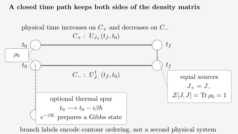
The closed time path represents both sides of density-matrix evolution. The $C_+$ branch carries $U$, the $C_-$ branch carries $U^\dagger$, and an optional vertical segment prepares $\rho_0\propto e^{-\beta\mathcal K_0}$. Equal sources make the two real-time evolutions cancel inside the trace.

Equal-source unitarity

If the two sources are equal,

$$J_+(t)=J_-(t)=J(t),$$

then

$$\begin{aligned} \mathcal Z[J,J] &= \operatorname{Tr} \left[ U_J(t_f,t_0) \rho_0 U_J^\dagger(t_f,t_0) \right] \\ &= \operatorname{Tr}\rho_0 \\ &= 1. \end{aligned}$$

This identity is a central diagnostic. It expresses trace preservation and unitarity before any approximation is made.

If an approximate closed-system calculation gives

$$\mathcal Z[J,J]\ne1,$$

then branch signs, normalization, source placement, or the approximation scheme require inspection.

The branches are not two physical systems

The labels $+$ and $-$ encode whether an insertion lies on the forward or backward part of one ordered contour. They do not introduce a second copy of the laboratory system.

This differs from thermo-field doubling, where an enlarged Hilbert space purifies a thermal density operator. Both constructions use doubled-looking notation, but their mathematical purposes are distinct.

The final time is auxiliary

Provided $t_f$ lies later than every insertion and the two branches are treated consistently, physical observables do not depend on its arbitrary value. Moving $t_f$ only extends a segment on which forward and backward unitary evolution cancels.

Contour Ordering

Let $z$ denote a point on the contour. Contour ordering $\mathcal T_C$ places the point encountered later along the directed contour to the left.

Every point on $C_-$ is later in contour order than every point on $C_+$, even when its numerical real-time coordinate is smaller. Along $C_+$, contour ordering agrees with ordinary time ordering. Along $C_-$, it agrees with anti-time ordering.

For a normal fermionic single-particle function,

$$G_C(z,z') = -\frac{i}{\hbar} \left\langle \mathcal T_C c(z)c^\dagger(z') \right\rangle.$$

Restricting each argument to a branch produces four components:

$$\mathbf G = \begin{pmatrix} G^{++} & G^{+-} \\ G^{-+} & G^{--} \end{pmatrix}.$$

With the convention fixed above,

$$\begin{aligned} G^{++} &= G^{\mathcal T}, & G^{--} &= G^{\widetilde{\mathcal T}}, \\ G^{+-} &= G^<, & G^{-+} &= G^>. \end{aligned}$$

Thus the apparent branch doubling packages four familiar orderings into one contour object.

Greater, Lesser, Retarded, Advanced, and Keldysh Components

The greater and lesser functions retain ordering and occupation information:

$$\begin{aligned} G^>(t,t') &= -\frac{i}{\hbar} \left\langle c(t)c^\dagger(t') \right\rangle, \\ G^<(t,t') &= +\frac{i}{\hbar} \left\langle c^\dagger(t')c(t) \right\rangle. \end{aligned}$$

The retarded and advanced functions are

$$\begin{aligned} G^{\mathrm R}(t,t') &= \theta(t-t') \\ &\qquad\times \left[ G^>(t,t')-G^<(t,t') \right], \\ G^{\mathrm A}(t,t') &= -\theta(t'-t) \\ &\qquad\times \left[ G^>(t,t')-G^<(t,t') \right]. \end{aligned}$$

The Keldysh component is commonly defined as

$$G^{\mathrm K}(t,t') = G^>(t,t')+G^<(t,t').$$

The time-ordered components can also be reconstructed:

$$\begin{aligned} G^{\mathcal T}(t,t') &= \theta(t-t')G^>(t,t') \\ &\qquad + \theta(t'-t)G^<(t,t'), \\ G^{\widetilde{\mathcal T}}(t,t') &= \theta(t'-t)G^>(t,t') \\ &\qquad + \theta(t-t')G^<(t,t'). \end{aligned}$$

Consequently, the four branch components are not all independent. One exact identity is

$$G^{++} + G^{--} = G^{+-} + G^{-+}.$$

It is a useful branch-bookkeeping check.

Equal-time occupation

The lesser function directly carries the one-body density matrix:

$$n(t) = \left\langle c^\dagger(t)c(t) \right\rangle = -i\hbar\,G^<(t,t).$$

For orbitals $a,b$,

$$n_{ba}(t) = -i\hbar\,G^<_{ab}(t,t).$$

A retarded propagator does not generally determine this matrix away from equilibrium.

Spectral versus statistical information

The difference

$$G^>-G^<$$

builds the retarded and advanced functions and therefore carries causal spectral propagation. The sum

$$G^>+G^<$$

builds $G^{\mathrm K}$ and carries statistical occupation information.

This language is exact as a decomposition. Calling one component purely “spectral” and the other purely “distributional” can become approximate in interacting, matrix-valued, or strongly time-dependent settings, so the operator definitions remain primary.

The Keldysh Rotation

Instead of the branch basis $(+,-)$, one often uses linear combinations adapted to physical and difference sources:

$$\begin{aligned} J_{\mathrm{cl}} &= \frac{J_++J_-}{2}, \\ J_{\mathrm q} &= J_+-J_-. \end{aligned}$$

Equal physical sources correspond to

$$J_{\mathrm q}=0.$$

The normalization identity becomes

$$\mathcal Z[J_{\mathrm{cl}},0]=1.$$

An analogous linear transformation reorganizes the branch Green functions into retarded, advanced, and Keldysh components. The exact placement of $G^{\mathrm R}$, $G^{\mathrm A}$, and $G^{\mathrm K}$ inside a rotated $2\times2$ matrix depends on the ordering of rotated fields and on factors of $2$. A formula copied from another source is safe only after its rotation matrix and source normalization are copied too.

The conceptual payoff is stable across conventions:

• retarded and advanced components encode causal propagation;
• the Keldysh or lesser component tracks statistical information;
• the vanishing difference source expresses normalization;
• mixed derivatives generate physical response.

Free Fermionic Mode Benchmark

Consider

$$H = \epsilon\,c^\dagger c$$

and an initial state with

$$n_0 = \langle c^\dagger c\rangle.$$

The Heisenberg operator is

$$c(t) = e^{-i\epsilon(t-t_0)/\hbar} c(t_0).$$

Let

$$\Delta t=t-t'.$$

Then

$$\begin{aligned} G^>(t,t') &= -\frac{i}{\hbar} (1-n_0) e^{-i\epsilon\Delta t/\hbar}, \\ G^<(t,t') &= +\frac{i}{\hbar} n_0 e^{-i\epsilon\Delta t/\hbar}. \end{aligned}$$

Their difference is

$$G^>(t,t')-G^<(t,t') = -\frac{i}{\hbar} e^{-i\epsilon\Delta t/\hbar},$$

so

$$G^{\mathrm R}(t,t') = -\frac{i}{\hbar} \theta(\Delta t) e^{-i\epsilon\Delta t/\hbar}.$$

The occupation $n_0$ cancels from the retarded function for this free canonical mode. It remains explicit in $G^<$ and $G^{\mathrm K}$:

$$G^{\mathrm K}(t,t') = -\frac{i}{\hbar} (1-2n_0) e^{-i\epsilon\Delta t/\hbar}.$$

This benchmark cleanly displays the information split:

• $G^{\mathrm R}$ and $G^{\mathrm A}$ describe the available propagation at energy $\epsilon$.
• $G^<$ and $G^{\mathrm K}$ retain the occupation $n_0$.

In an interacting system, the retarded self-energy can itself depend on the evolving state. The simple cancellation of $n_0$ is therefore a benchmark, not a universal independence theorem.

Equilibrium Closes the Component Hierarchy

For the free fermionic mode in equilibrium,

$$n_0=f(\epsilon), \qquad f(E) = \frac{1}{e^{\beta E}+1}.$$

In the energy-domain convention of the neighboring Green-function pages,

$$\begin{aligned} G^<(E) &= 2\pi i\, f(E)A(E), \\ G^>(E) &= -2\pi i\, [1-f(E)]A(E). \end{aligned}$$

Therefore,

$$\begin{aligned} G^{\mathrm K}(E) &= [1-2f(E)] \\ &\qquad\times \left[ G^{\mathrm R}(E)-G^{\mathrm A}(E) \right]. \end{aligned}$$

Since

$$1-2f(E) = \tanh \left( \frac{\beta E}{2} \right),$$

the equilibrium statistical component is fixed by temperature and the spectral discontinuity.

This is a fermionic fluctuation–dissipation relation in the declared convention. Bosonic fields involve the corresponding Bose factor and a hyperbolic cotangent. Observable commutator and symmetrized correlators have their own normalization.

Away from equilibrium, one generally cannot replace the distribution by a single function $f(E)$ or a single effective temperature. One must propagate or otherwise determine $G^<$, $G^{\mathrm K}$, a density matrix, or an equivalent statistical object.

Thermal Initial States and the Imaginary Spur

A closed real-time contour can begin with any explicitly specified $\rho_0$. If the initial state is thermal,

$$\rho_0 = \frac{e^{-\beta\mathcal K_0}}{\mathcal Z_0},$$

the Gibbs factor can be represented by an additional vertical contour segment:

$$t_0 \longrightarrow t_0-i\beta\hbar.$$

The combined contour contains:

1. a forward real-time branch from $t_0$ to $t_f$;
2. a backward real-time branch from $t_f$ to $t_0$;
3. an imaginary-time branch encoding the thermal preparation.

This extension is often called the Konstantinov–Perel contour.

Why the spur matters

The imaginary branch can encode correlations already present in the interacting thermal initial state. Replacing that state by a Gaussian density operator while keeping only a real-time contour changes the problem unless initial correlations are restored by boundary terms or initial-correlation insertions.

When it can be omitted

The spur need not be drawn when:

• $\rho_0$ is supplied exactly as an operator or matrix;
• a pure initial state is imposed directly;
• the initial state is Gaussian and fully encoded by its covariance in the chosen method;
• an approximation deliberately neglects initial correlations and states that assumption.

Omitting the segment is a representation choice only when the same initial state is still encoded elsewhere.

Example: A Sudden Spin Quench

Prepare a spin-$1/2$ at $t_0$ in

$$\rho_0 = |\uparrow_z\rangle \langle\uparrow_z|.$$

For $t\gt t_0$, let

$$H_f = \frac{\hbar\Omega}{2} \sigma_x.$$

The evolution operator is

$$U(t,t_0) = \exp \left[ -\frac{i\Omega(t-t_0)}{2} \sigma_x \right].$$

Using the Pauli algebra,

$$\begin{gathered} U^\dagger(t,t_0) \sigma_z U(t,t_0) \\ = \sigma_z \cos[\Omega(t-t_0)] \\ + \sigma_y \sin[\Omega(t-t_0)]. \end{gathered}$$

Taking the expectation value in $|\uparrow_z\rangle$ gives

$$\langle\sigma_z(t)\rangle = \cos[\Omega(t-t_0)].$$

The preparation axis and post-quench Hamiltonian axis are independent inputs. A thermal circle generated only by $H_f$ would instead prepare a state diagonal in the $\sigma_x$ basis. It would not encode the chosen $|\uparrow_z\rangle$ preparation.

Forward–backward reading

The same answer can be written as

$$\langle\sigma_z(t)\rangle = \operatorname{Tr} \left[ U(t,t_0) \rho_0 U^\dagger(t,t_0) \sigma_z \right].$$

The two real-time branches are already visible. A contour source coupled to $\sigma_z$ would generate this expectation and its ordered correlation functions by functional differentiation.

What this example does not show

The isolated two-level system has no irreversible relaxation. Its oscillations recur forever. Damping requires additional degrees of freedom, averaging, a continuum, an open-system approximation, or a thermodynamic limit. A decaying fit cannot be inferred from the contour notation alone.

Stationarity, Periodicity, and Steady States

These three ideas should not be conflated.

Equilibrium stationarity

If

$$[H,\rho_\beta]=0,$$

then correlation functions are invariant under a common real-time shift:

$$C(t+s,t'+s) = C(t,t').$$

KMS additionally relates operator orderings across an imaginary-time displacement.

Periodically driven states

For

$$H(t+\mathcal T)=H(t),$$

a long-time state may become periodic:

$$C(t+\mathcal T,t'+\mathcal T) = C(t,t').$$

This is discrete time-translation covariance, not thermal equilibrium. A Floquet state need not satisfy a Gibbs KMS relation.

Nonequilibrium steady states

A driven open system can approach time-independent one-time observables while sustaining nonzero currents and entropy production. Such a steady state can be stationary without being equilibrium. Detailed balance and fluctuation–dissipation relations must be checked, not assumed.

Interacting Systems: What the Contour Organizes

For an interacting theory, the contour Green function satisfies the schematic Dyson equation

$$G = G_0 + G_0 \star_C \Sigma \star_C G,$$

where

$$(A\star_C B)(z,z') = \int_C d\bar z\, A(z,\bar z) B(\bar z,z').$$

Every internal integration follows the directed contour. The self-energy $\Sigma$ is itself a contour object.

Projecting this equation onto real-time components produces coupled equations for $G^{\mathrm R}$, $G^{\mathrm A}$, $G^<$, and related objects. Those projections lead to the Kadanoff–Baym equations and, after additional assumptions, to kinetic or quantum Boltzmann equations.

This preview stops before deriving those rules. Three lessons are nevertheless important:

1. the retarded equation alone does not close the nonequilibrium problem;
2. initial conditions enter the two-time equations explicitly;
3. approximations to $\Sigma$ must be chosen consistently across components.

Memory

A typical projected equation contains a history integral:

$$\begin{aligned} & \int_{t_0}^{t} d\bar t\, \Sigma^{\mathrm R}(t,\bar t) G^<(\bar t,t') \\ &\quad + \int_{t_0}^{t'} d\bar t\, \Sigma^<(t,\bar t) G^{\mathrm A}(\bar t,t'). \end{aligned}$$

Its value depends on earlier times. Replacing it by a local collision term is a Markov or kinetic approximation, not an identity.

Conserving approximations

An arbitrary mixture of a dressed retarded propagator and an unrelated lesser self-energy can violate particle number, energy, or Ward identities. Self-consistent functionals of Baym–Kadanoff type provide one route to conserving approximations, although self-consistency does not by itself guarantee numerical accuracy or a controlled expansion.

Closed Systems, Open Systems, and Reservoirs

The same forward–backward logic appears in several settings, but the dynamical object changes.

Isolated closed system

For a finite isolated system,

$$\rho(t) = U(t,t_0)\rho_0U^\dagger(t,t_0)$$

is exact. Apparent relaxation can arise through dephasing of many frequencies, but the fine-grained von Neumann entropy remains constant:

$$S[\rho(t)] = -k_{\mathrm B} \operatorname{Tr} \left[ \rho(t)\ln\rho(t) \right] = S[\rho_0].$$

Reduced open system

If a system $S$ is coupled to an environment $E$,

$$\rho_S(t) = \operatorname{Tr}_E \left[ U_{SE}(t,t_0) \rho_{SE,0} U_{SE}^\dagger(t,t_0) \right].$$

Tracing out $E$ couples the two branches through an influence functional. Markovian master equations arise only after assumptions about initial correlations, reservoir memory, coupling strength, and time scales.

Transport reservoirs

For reservoirs at different temperatures or chemical potentials, the initial state may be assembled from separately equilibrated sectors and then coupled. The steady current depends on both spectral transmission and reservoir distribution functions. Equilibrium KMS closure for one global temperature is unavailable.

Method-Selection Guide

Ask these questions in order.

Is the state equilibrium and stationary?

If yes, imaginary-time, Matsubara, spectral, and retarded methods are often sufficient. Choose the representation best matched to the observable and numerical method.

Is the perturbation weak?

If yes, Kubo response may answer the question without propagating the full state. Check whether first order is adequate and whether heating or occupation changes matter.

Is the Hilbert space small enough for direct propagation?

If yes, exact diagonalization, Krylov propagation, or direct integration of the Schrödinger or von Neumann equation may be clearer than a contour field theory.

Are two-time correlations or interacting transients required?

If yes, nonequilibrium Green functions, tensor-network real-time evolution, stochastic methods, or another explicit initial-value framework may be needed. The contour is one organizing language, not the only algorithm.

Is the system open?

State the system–environment partition and justify the reduced-dynamics approximation. A Lindblad equation, hierarchical method, influence functional, or explicit reservoir treatment answers different regimes.

Is a continuum field theory essential?

When renormalization, relativistic fields, hydrodynamic effective actions, gauge structure, or full contour diagrammatics become central, use Continue on QFT.org to select the planned destination and current live fallback.

Diagnostics and Consistency Checks

Trace and normalization

For a closed system,

$$\operatorname{Tr}\rho(t)=1.$$

In the source formulation,

$$\mathcal Z[J,J]=1.$$

Hermiticity and positivity

The density operator must satisfy

$$\rho(t)=\rho^\dagger(t), \qquad \rho(t)\geq0.$$

Approximate one-body closures can preserve some conservation laws while violating positivity, so both properties require independent checks.

Causality

A retarded quantity must vanish before its perturbation:

$$G^{\mathrm R}(t,t')=0 \qquad \text{for }t\lt t'.$$

In a stable stationary problem, its frequency representation must have the corresponding analytic half-plane.

Equal-time algebra

For one canonical fermionic mode,

$$\langle cc^\dagger\rangle + \langle c^\dagger c\rangle = 1.$$

In Green-function language,

$$i\hbar\,G^>(t,t) -i\hbar\,G^<(t,t) = 1.$$

Equal-time identities expose branch signs and discretization errors quickly.

Equilibrium recovery

If the drive is removed and the initial state is Gibbs for the same Hamiltonian, the calculation should recover:

• time-translation invariance;
• KMS boundary relations;
• detailed balance;
• fluctuation–dissipation relations;
• equilibrium Matsubara and retarded limits.

Conservation laws

For a time-independent isolated Hamiltonian,

$$\frac{d}{dt} \langle H\rangle = 0.$$

If $[H,N]=0$,

$$\frac{d}{dt} \langle N\rangle = 0.$$

During an explicit drive, energy need not be conserved. The correct check is the power balance determined by $\partial H/\partial t$.

Independence of the contour turn

Physical results should not change when $t_f$ is moved later than all insertions. Residual dependence indicates incomplete branch cancellation or an inconsistent truncation.

Common Mistakes

• Treating analytic continuation as a procedure that creates arbitrary nonequilibrium occupations.
• Assuming every stationary state is thermal.
• Using a retarded propagator alone to infer an equal-time density matrix.
• Forgetting that $\rho_0$ and the post-preparation Hamiltonian are separate inputs.
• Reading $+$ and $-$ as two physical copies of the system.
• Giving both branches the same exponential sign while ignoring the reversed contour orientation.
• Setting $J_+=J_-$ before taking the derivatives needed to generate observables.
• Mixing branch, retarded–advanced, and Keldysh bases without declaring the rotation.
• Copying a bosonic fluctuation–dissipation factor into a fermionic convention.
• Dropping the imaginary spur while silently discarding correlated thermal initial conditions.
• Assuming a Markovian collision term when the exact equation contains memory.
• Combining self-energies from incompatible approximations and then claiming exact conservation.
• Calling dephasing in a finite closed system irreversible thermalization.
• Inferring a temperature from one fitted observable without testing KMS or fluctuation–dissipation consistency.
• Forgetting that a full real-time calculation can be more expensive than an equilibrium Matsubara calculation because two time arguments must be retained.

Practical Workflow

1. State the preparation. Specify $\rho_0$, its correlations, and whether it is pure, Gibbs, generalized Gibbs, or otherwise constructed.
2. State the protocol. Give $H(t)$, switching times, source signs, and any reservoir couplings.
3. Choose the target. Distinguish one-time observables, retarded response, noise, spectra, occupations, and full counting statistics.
4. Use the smallest sufficient method. Direct propagation can be preferable for small systems; linear response can be preferable for weak probes.
5. Declare contour conventions. Fix branch direction, Green-function signs, source rotation, and Fourier units.
6. Encode initial correlations. Use an explicit density operator, covariance, imaginary spur, or justified approximation.
7. Check exact identities. Test normalization, causality, equal-time algebra, symmetries, and conserved quantities.
8. Recover equilibrium. Turn off the drive and verify KMS and fluctuation–dissipation limits.
9. Report approximation boundaries. State memory, gradient, weak-coupling, quasiparticle, Markov, or truncation assumptions.

Exercises

Exercise 1: Equal-source normalization

Starting from

$$\mathcal Z[J_+,J_-] = \operatorname{Tr} \left[ U_{J_+} \rho_0 U_{J_-}^\dagger \right],$$

prove that $\mathcal Z[J,J]=1$ for a normalized closed-system initial state. Which assumptions enter?

Solution

Set the two source histories equal:

$$U_{J_+}=U_{J_-}=U_J.$$

Then

$$\begin{aligned} \mathcal Z[J,J] &= \operatorname{Tr} \left[ U_J\rho_0U_J^\dagger \right] \\ &= \operatorname{Tr} \left[ \rho_0U_J^\dagger U_J \right] \\ &= \operatorname{Tr}\rho_0 \\ &= 1. \end{aligned}$$

The second line uses cyclicity of the trace, the third uses unitary evolution, and the fourth uses normalization of $\rho_0$.

The identity can fail if evolution is represented by a nonunitary effective operator without the corresponding environment or jump terms, if the two branches use inconsistent Hamiltonians, or if an approximation violates trace preservation.

Exercise 2: Reconstruct the branch functions

Use the definitions of $G^>$ and $G^<$ to show that

$$G^{\mathcal T} = \theta(t-t')G^> + \theta(t'-t)G^<$$

and

$$G^{\widetilde{\mathcal T}} = \theta(t'-t)G^> + \theta(t-t')G^<.$$

Deduce

$$G^{++}+G^{--} = G^{+-}+G^{-+}.$$

Solution

Ordinary time ordering places the later operator to the left. For $t\gt t'$, the ordered product has the greater ordering; for $t'\gt t$, exchanging the fermionic fields produces the lesser convention. Therefore

$$G^{\mathcal T} = \theta(t-t')G^> + \theta(t'-t)G^<.$$

Anti-time ordering reverses the cases:

$$G^{\widetilde{\mathcal T}} = \theta(t'-t)G^> + \theta(t-t')G^<.$$

Adding and using

$$\theta(t-t') + \theta(t'-t) = 1$$

away from coincident times gives

$$G^{\mathcal T} + G^{\widetilde{\mathcal T}} = G^>+G^<.$$

With

$$\begin{aligned} G^{++} &= G^{\mathcal T}, & G^{--} &= G^{\widetilde{\mathcal T}}, \\ G^{+-} &= G^<, & G^{-+} &= G^>, \end{aligned}$$

the branch identity follows. At coincident times, use one declared ordering prescription consistently.

Exercise 3: Occupation is not in the free retarded propagator

For the free fermionic mode

$$H=\epsilon c^\dagger c,$$

derive $G^{\mathrm R}$ and $G^<$ for an arbitrary initial occupation $n_0$. Explain why two states with different $n_0$ can have the same retarded propagator.

Solution

The Heisenberg solution is

$$c(t) = e^{-i\epsilon(t-t_0)/\hbar}c(t_0).$$

Thus

$$G^<(t,t') = \frac{i}{\hbar} n_0 e^{-i\epsilon(t-t')/\hbar}.$$

The anticommutation relation gives

$$\langle cc^\dagger\rangle = 1-n_0,$$

so

$$G^>(t,t') = -\frac{i}{\hbar} (1-n_0) e^{-i\epsilon(t-t')/\hbar}.$$

Their difference is independent of $n_0$:

$$G^>-G^< = -\frac{i}{\hbar} e^{-i\epsilon(t-t')/\hbar}.$$

Therefore

$$G^{\mathrm R}(t,t') = -\frac{i}{\hbar} \theta(t-t') e^{-i\epsilon(t-t')/\hbar}.$$

The free retarded function records the available canonical mode and its energy. The lesser function records whether the mode is occupied. In interacting systems, state-dependent self-energies can make even the retarded spectrum depend on the evolving distribution.

Exercise 4: Why a quench is not one thermal circle

A system begins in

$$\rho_0 = \frac{e^{-\beta H_i}}{\mathcal Z_i}$$

and evolves for $t\gt t_0$ under $H_f$, with

$$[H_i,H_f]\ne0.$$

Explain why replacing the problem by a Matsubara calculation generated by $H_f$ changes the initial state.

Solution

A Matsubara circle generated by $H_f$ represents

$$\rho_f^{\mathrm{eq}} = \frac{e^{-\beta H_f}}{\mathcal Z_f}.$$

The actual initial state is

$$\rho_0 = \frac{e^{-\beta H_i}}{\mathcal Z_i}.$$

When $[H_i,H_f]\ne0$, these operators generally have different eigenvectors as well as different weights. In particular,

$$[H_f,\rho_0]\ne0$$

generically, so the actual state evolves and is not stationary under $H_f$. Replacing it by $\rho_f^{\mathrm{eq}}$ removes the quench and substitutes a different physical preparation.

A combined contour may use an imaginary spur generated by $H_i$ to prepare $\rho_0$ and real branches generated by $H_f$ to propagate it.

Exercise 5: Retarded response versus state propagation

For a pulse

$$H_{\mathrm{pert}}(t) = -\lambda\,\delta(t-t_p)B,$$

use linear response to find the first-order change in $\langle A(t)\rangle$. Why does this not determine the full post-pulse density operator?

Solution

Insert

$$f(t') = \lambda\,\delta(t'-t_p)$$

into

$$\delta\langle A(t)\rangle = \int_{t_0}^{t} dt'\, \chi^{\mathrm R}_{AB}(t,t')f(t').$$

The result is

$$\delta\langle A(t)\rangle = \lambda\, \chi^{\mathrm R}_{AB}(t,t_p)$$

for $t\gt t_p$, and zero for $t\lt t_p$.

This determines one observable to first order in $\lambda$. The full density operator contains all orders in the pulse, all operator channels, coherences, and occupation changes. Reconstructing it would require a tomographically complete set of observables or direct propagation of the state.

Exercise 6: Thermal closure of the free mode

For the free fermionic benchmark, set

$$n_0=f(\epsilon).$$

Show that

$$G^{\mathrm K} = (1-2f) (G^{\mathrm R}-G^{\mathrm A})$$

in energy space. What fails if $n_0$ is arbitrary?

Solution

The equilibrium greater and lesser functions are

$$\begin{aligned} G^>(E) &= -2\pi i [1-f(E)]A(E), \\ G^<(E) &= +2\pi i f(E)A(E). \end{aligned}$$

Adding gives

$$G^{\mathrm K}(E) = -2\pi i [1-2f(E)]A(E).$$

The spectral discontinuity is

$$G^{\mathrm R}(E)-G^{\mathrm A}(E) = -2\pi i A(E).$$

Therefore

$$\begin{aligned} G^{\mathrm K}(E) &= [1-2f(E)] \\ &\qquad\times \left[ G^{\mathrm R}(E)-G^{\mathrm A}(E) \right]. \end{aligned}$$

For an arbitrary stationary free-mode occupation $n_0$, the same algebra holds with $f(\epsilon)$ replaced by $n_0$ at that mode. What fails is the claim that one temperature and chemical potential determine the statistical factor. For a general nonequilibrium many-mode state, there may be no universal scalar $f(E)$ at all.

Exercise 7: Diagnose an inconsistent result

A numerical closed-system calculation reports all three:

$$\mathcal Z[J,J]=0.997,$$ $$G^{\mathrm R}(t,t')\ne0 \quad \text{for }t\lt t',$$

and

$$\operatorname{Tr}\rho(t)=1.$$

Can the last equality certify the calculation? List likely sources of the other failures.

Solution

No. Trace normalization of the propagated density matrix is one check, but it does not certify source normalization or causal ordering.

The failure

$$\mathcal Z[J,J]\ne1$$

can arise from:

• inconsistent source signs on the two branches;
• unequal discretization or truncation of forward and backward evolution;
• a missing normalization denominator;
• an approximate influence functional or self-energy that is not trace preserving;
• evaluating the branches with different Hamiltonians unintentionally.

The acausal retarded component can arise from:

• exchanging retarded and advanced definitions;
• a reversed Fourier prescription;
• incorrect step functions;
• mixing branch components with the wrong Keldysh rotation;
• time-grid interpolation that leaks support;
• a self-energy projection inconsistent with the Green-function projection.

Each exact identity tests a different part of the implementation. Passing one does not excuse failure of another.

Exercise 8: Choose the sufficient method

Choose the smallest sufficient method for each task:

1. the equilibrium heat capacity of an interacting lattice model;
2. the linear conductivity induced by a weak probe;
3. the exact magnetization after a sudden pulse in a ten-dimensional Hilbert space;
4. the evolving particle distribution after an interacting quench;
5. the reduced dynamics of a weakly coupled system in a short-memory thermal reservoir.

Solution

1. Use equilibrium statistical mechanics, imaginary time, or another partition-function method. A real-time contour is unnecessary unless it is computationally advantageous.
2. Use the Kubo formula and a retarded current response, provided the probe is weak and the reference state is stationary.
3. Propagate the finite-dimensional state or density matrix directly. This is simpler than introducing a field-theory contour.
4. Use an explicit nonequilibrium initial-value method that carries occupations and correlations, such as nonequilibrium Green functions, tensor-network real-time evolution, or another controlled many-body method suited to the model.
5. A justified Markovian master equation may suffice if weak coupling, short reservoir memory, and the required secular or positivity conditions hold. Otherwise retain a non-Markovian influence-functional or explicit-reservoir treatment.

The contour is conceptually general, but “general” does not mean “always computationally best.”

Cross-Links

• Finite-Temperature QM Overview – the equilibrium representation map and method-selection context.
• KMS Condition Preview – the equilibrium condition that closes thermal ordering relations.
• Matsubara Formalism Preview – compact imaginary time, discrete thermal frequencies, and equilibrium loop sums.
• Analytic Continuation – exact boundary values and numerical real-frequency inference from Euclidean data.
• Thermal Green Functions – imaginary-time ordering, contact jumps, and free thermal benchmarks.
• Retarded and Advanced Response – causal support, analytic structure, dispersion relations, and stability.
• Green Functions in Many-Body QM – single-particle greater, lesser, retarded, advanced, and spectral conventions.
• Time-Dependent Correlations – stationarity, dephasing, recurrence, and finite-time spectra.
• Diagrammatic Methods Preview – graph conventions, self-energies, Dyson equations, and the boundary of contour diagrammatics.
• Thermal Density Operators – Gibbs states, normalization, entropy, and ensemble meaning.
• Correlation Functions in Path Integrals – source derivatives and ordered insertions in path-integral language.
• Why Many-Body QM Leads to QFT – the broader move from many-body operators to fields and generating functionals.
• Schwinger–Keldysh Bridge – doubled fields, in-in effective actions, influence functionals, and the handoff to nonequilibrium QFT.
• Continue on QFT.org – publication-aware route to full Schwinger–Keldysh field theory, contour diagrammatics, and effective descriptions.

References

1. J. Schwinger, “Brownian Motion of a Quantum Oscillator”, Journal of Mathematical Physics 2, 407–432 (1961).
2. L. V. Keldysh, “Diagram Technique for Nonequilibrium Processes”, Soviet Physics JETP 20, 1018–1026 (1965).
3. R. Kubo, “Statistical-Mechanical Theory of Irreversible Processes. I”, Journal of the Physical Society of Japan 12, 570–586 (1957).
4. L. P. Kadanoff and G. Baym, Quantum Statistical Mechanics: Green’s Function Methods in Equilibrium and Nonequilibrium Problems, W. A. Benjamin (1962).
5. G. Baym, “Self-Consistent Approximations in Many-Body Systems”, Physical Review 127, 1391–1401 (1962).
6. P. Danielewicz, “Quantum Theory of Nonequilibrium Processes, I”, Annals of Physics 152, 239–304 (1984).
7. J. Rammer, Quantum Field Theory of Non-equilibrium States, Cambridge University Press (2007).
8. A. Kamenev, Field Theory of Non-Equilibrium Systems, 2nd ed., Cambridge University Press (2023).
9. G. Stefanucci and R. van Leeuwen, Nonequilibrium Many-Body Theory of Quantum Systems, 2nd ed., Cambridge University Press (2025).
10. H. Aoki, N. Tsuji, M. Eckstein, M. Kollar, T. Oka, and P. Werner, “Nonequilibrium Dynamical Mean-Field Theory and Its Applications”, Reviews of Modern Physics 86, 779–837 (2014).