Schwinger–Keldysh Bridge

The Schwinger–Keldysh formalism is the field-theory language for finite-time expectation values, response, fluctuations, and reduced dynamics in a specified initial state. It is an in-in construction: both the amplitude and its conjugate begin in the same density operator, evolve along opposite branches of a closed time path, and are sewn together after the latest operator insertion.

In natural units, its generating functional is

$$\begin{aligned} Z[J_+,J_-] &= \operatorname{Tr} \Bigl[ U_{J_+}(t_f,t_0) \\ &\qquad\times \rho_0 U_{J_-}^{\dagger}(t_f,t_0) \Bigr]. \end{aligned}$$

When the two sources agree, unitarity closes the evolution:

$$Z[J,J] = \operatorname{Tr}\rho_0 = 1.$$

That identity is not merely a normalization chosen after a calculation. It organizes the doubled fields, removes unobservable vacuum pieces, constrains effective actions, and supplies some of the strongest diagnostics available in nonequilibrium QFT.

The Real-Time Thermal Dynamics Preview is the canonical home for why the path closes, the four branch orderings, greater and lesser functions, and elementary many-body examples. This page starts at the next layer: what changes when each branch carries a quantum field, when modes interact through local vertices, when environmental fields are integrated out, and when renormalization and symmetry constraints become unavoidable.

Purpose and Canonical Scope

This page owns the bridge from closed-time-path many-body mechanics to nonequilibrium field theory. It develops:

• the distinction between in-out amplitudes and in-in expectation values;
• the doubled field path integral and its initial-state boundary kernel;
• one explicit average/difference, or r/a, convention;
• the response–fluctuation organization of bosonic two-point functions;
• branch signs and doubled interaction vertices;
• the in-in one-particle-irreducible effective action;
• influence functionals, dissipation, noise, and stochastic limits;
• the route from contour Dyson equations to two-time, kinetic, and hydrodynamic descriptions;
• ultraviolet, initial-state, gauge, and long-time consistency issues;
• the boundary at which a full QFT treatment is needed.

Neighboring pages retain their own canonical material:

• Real-Time Thermal Dynamics Preview owns the operator derivation of the closed path and the branch-component dictionary.
• From Sources in QM to Generating Functionals in QFT owns generic source differentiation, connected generators, and the in-out vacuum construction.
• From QM Path Integrals to Field Path Integrals owns the replacement of trajectories by field histories and the spacetime functional measure.
• Finite-Temperature QFT Bridge owns thermal circles, Matsubara loop sums, screening, and equilibrium analytic continuation.
• Diagrammatic Methods Preview owns ordinary graph combinatorics, line and vertex bookkeeping, and the elementary Dyson equation.
• Reduced Dynamics owns partial traces, dynamical maps, complete positivity, and the system-level meaning of an environment.

The aim is not to compress all of nonequilibrium QFT into one article. It is to make the mathematical handoff precise enough that the doubled notation, causal structure, and limitations are recognizable when they reappear in a full field-theory treatment.

Convention Ledger

This subject has several internally consistent sign and normalization conventions. A matrix copied without its field rotation and source coupling is not a formula; it is an invitation to a sign error. The conventions below remain fixed throughout the page.

Units, spacetime, and fields

Set

$$\hbar = c = k_{\mathrm B} = 1.$$

A spacetime point is

$$x = (x^0,\mathbf x), \qquad \int_x \equiv \int_{t_0}^{t_f} dx^0 \int d^d\mathbf x.$$

Most explicit formulas use a real bosonic field $\phi$. Complex fields, fermions, Nambu multiplets, and gauge fields require the appropriate conjugation, Grassmann, or constraint structure. The doubled-contour principle survives those changes, but individual matrix entries and signs need not.

Source coupling

On the two real-time branches, use

$$\begin{aligned} S_J &= S[\phi_+] - S[\phi_-] \\ &\quad+ \int_x \left( J_+\phi_+ - J_-\phi_- \right). \end{aligned}$$

The corresponding Hamiltonian perturbation is $H_{\mathrm{pert}}=-\int d^d\mathbf x\,J\phi$. With this choice, the response convention is

$$\chi_R(x,y) = i\theta(x^0-y^0) \left\langle [\phi(x),\phi(y)] \right\rangle.$$

Many QFT texts instead call $-i\theta\langle[\phi,\phi]\rangle$ the retarded Green function. That definition is valid, but its source-response sign and the r/a matrix below change accordingly.

Average and difference variables

Define

$$\begin{aligned} \phi_r &= \frac{\phi_++\phi_-}{2}, & \phi_a &= \phi_+-\phi_-, \\ J_r &= \frac{J_++J_-}{2}, & J_a &= J_+-J_-. \end{aligned}$$

Then

$$J_+\phi_+ - J_-\phi_- = J_a\phi_r + J_r\phi_a.$$

Equal physical sources mean

$$J_a=0, \qquad J_r=J.$$

The labels $r/a$, classical/quantum, $1/2$, and average/difference all occur in the literature. Some authors divide both rotated fields by $\sqrt2$; others put the factor $1/2$ in the difference variable. Those alternatives move factors of two among propagators, sources, and vertices.

Fourier transform

For a stationary two-point function,

$$G(\omega,\mathbf k) = \int dt \int d^d\mathbf x\, e^{i\omega t-i\mathbf k\cdot\mathbf x} G(t,\mathbf x).$$

Outside stationarity, two time arguments remain independent until a Wigner transform or another controlled approximation is introduced.

Why In-In Is Different from In-Out

An in-out object has the schematic form

$$Z_{\mathrm{out,in}}[J] = \langle\Omega_{\mathrm{out}}| U_J |\Omega_{\mathrm{in}}\rangle.$$

Its derivatives generate time-ordered matrix elements between asymptotic states. That architecture is ideal for scattering amplitudes, vacuum persistence, and S-matrix observables. It is not, by itself, a finite-time expectation value in a density operator.

The in-in question is instead

$$\langle O(t)\rangle = \operatorname{Tr} \left[ \rho_0 U^{\dagger}(t,t_0) O U(t,t_0) \right].$$

The same initial state appears in the amplitude and its conjugate. Consequently:

• the initial density matrix is physical input rather than an asymptotic boundary condition;
• expectation values are real when the inserted operator is Hermitian;
• causal response emerges from cancellations between the branches;
• occupation and fluctuation data survive independently of retarded propagation;
• the result can follow quenches, drives, expansion, or environmental coupling.

Replacing an in-in calculation by an in-out one can produce complex or acausal-looking “equations of motion” for an expectation value. The algebra may be correct for an amplitude while answering the wrong physical question.

From the Trace to Doubled Fields

Insert field eigenstates at the initial and final times. The initial density operator becomes the kernel

$$\rho_0[\phi_{+0},\phi_{-0}] = \langle\phi_{+0}| \rho_0 |\phi_{-0}\rangle.$$

The generating functional can then be written

$$\begin{aligned} Z[J_+,J_-] &= \int \mathcal D\phi_+ \mathcal D\phi_- \, \rho_0[\phi_{+0},\phi_{-0}] \\ &\quad\times \delta[\phi_+(t_f)-\phi_-(t_f)] \\ &\quad\times \exp \left\{ iS[\phi_+] -iS[\phi_-] \right. \\ &\qquad\left. +i\int_x \left( J_+\phi_+ -J_-\phi_- \right) \right\}. \end{aligned}$$

The delta functional sews the two histories together at $t_f$. It implements the trace over the final field configuration. The turn time is auxiliary: if it lies after every insertion, exact observables cannot depend on where it is placed.

The pair $\phi_+,\phi_-$ does not describe two independent physical universes. It records the amplitude and conjugate-amplitude histories required by a probability or expectation value. Equal branch configurations cancel their microscopic phases:

$$S[\phi]-S[\phi]=0.$$

That cancellation becomes the r/a statement that an exact unitary action vanishes when $\phi_a=0$.

Initial correlations are boundary data

A useful representation is

$$\rho_0[\phi_{+0},\phi_{-0}] = \mathcal N e^{iS_0[\phi_{+0},\phi_{-0}]}.$$

A Gaussian $S_0$ specifies one- and two-point initial data. Cubic and higher terms encode non-Gaussian initial correlations and act as vertices localized on the initial surface. Setting those terms to zero is an assumption about state preparation, not a consequence of the contour.

For a thermal state, one may append an imaginary-time segment of length $\beta$ that prepares $e^{-\beta H}$. The Finite-Temperature QFT Bridge explains the equilibrium circle and KMS condition. A generic nonequilibrium $\rho_0$ need not admit that thermal representation.

The Closed-Time-Path Architecture

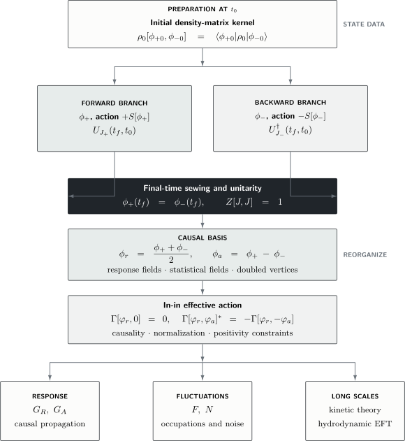
The field-theory layers of the Schwinger–Keldysh construction. The two action phases are sewn at the final time, reorganized into average and difference fields, and constrained before response, fluctuation, kinetic, or effective-theory information is extracted.

The figure emphasizes three logically distinct operations:

1. Prepare: specify $\rho_0$, including any correlations needed at $t_0$.
2. Double and sew: evolve an amplitude and its conjugate with branch-dependent fields and sources.
3. Reorganize: rotate to variables in which normalization, response, and fluctuations are transparent.

The final outputs are not interchangeable. $G_R$ answers a causal-response question; $F$ carries symmetrized fluctuation data; a kinetic or hydrodynamic description additionally requires scale separation and a controlled reduction.

The r/a Action and Its Vertices

Substitute

$$\phi_+ = \phi_r+\frac{\phi_a}{2}, \qquad \phi_- = \phi_r-\frac{\phi_a}{2}.$$

For a differentiable action,

$$\begin{aligned} S[\phi_+]-S[\phi_-] &= \int_x \phi_a(x) \frac{\delta S}{\delta\phi_r(x)} \\ &\quad +O(\phi_a^3). \end{aligned}$$

The term linear in $\phi_a$ contains the classical field equation. Higher odd powers retain quantum vertices. A closed microscopic bosonic action contains no term with zero $a$ fields because the two branches cancel at $\phi_a=0$.

Quartic example

For

$$S[\phi] = \int_x \left[ \frac12 \partial_\mu\phi \partial^\mu\phi - \frac{m^2}{2}\phi^2 - \frac{\lambda}{4!}\phi^4 \right],$$

the interaction difference follows from

$$\phi_+^4- \phi_-^4 = 4\phi_r^3\phi_a + \phi_r\phi_a^3.$$

Thus

$$\begin{aligned} S_{\mathrm{int},+} -S_{\mathrm{int},-} &= -\frac{\lambda}{4!} \int_x \left( 4\phi_r^3\phi_a + \phi_r\phi_a^3 \right). \end{aligned}$$

The $\phi_r^3\phi_a$ vertex survives in a classical statistical limit. The $\phi_r\phi_a^3$ vertex is intrinsically quantum in the usual $\hbar$ power counting. Dropping it can define a useful approximation in highly occupied weakly coupled regimes, but it is not an exact identity.

Branch-basis signs

Before rotation, every interaction vertex carries a branch label. A $+$-branch vertex inherits the phase from $+iS[\phi_+]$; the corresponding $-$-branch vertex inherits the opposite phase from $-iS[\phi_-]$. Internal branch labels are summed and propagator lines form a $2\times2$ contour matrix.

This doubled bookkeeping ensures that vacuum diagrams cancel at equal sources and that causal combinations emerge only after all required branch assignments are included. Keeping only the forward branch generally destroys those cancellations.

Sources, Mean Fields, and Physical Insertions

Define the connected generator

$$W[J_r,J_a] = -i\ln Z[J_r,J_a].$$

With the source convention above,

$$\begin{aligned} \varphi_r(x) &= \frac{\delta W}{\delta J_a(x)}, \\ \varphi_a(x) &= \frac{\delta W}{\delta J_r(x)}. \end{aligned}$$

At equal physical sources,

$$J_a=0, \qquad \varphi_a=0.$$

The physical expectation value is $\varphi_r$. A derivative with respect to $J_r$ perturbs the same source on both branches and inserts a difference field. That mixed derivative is why the r/a basis exposes causal response:

$$\frac{\delta\varphi_r(x)} {\delta J_r(y)} = \chi_R(x,y).$$

Pure derivatives with respect to $J_a$ generate symmetrized statistical correlations. Pure $J_r$ derivatives vanish at $J_a=0$ when they would represent only difference-field insertions. These statements assume the declared source normalization; changing the rotation changes the numerical factors.

Response and Fluctuation Components

For a real bosonic field, define

$$F(x,y) = \frac12 \left\langle \{\phi(x),\phi(y)\} \right\rangle_c,$$

and

$$\begin{aligned} \chi_R(x,y) &= i\theta(x^0-y^0) \langle[\phi(x),\phi(y)]\rangle, \\ \chi_A(x,y) &= -i\theta(y^0-x^0) \langle[\phi(x),\phi(y)]\rangle. \end{aligned}$$

The contour expectation values in the chosen r/a normalization obey

$$\begin{aligned} \langle\phi_r(x)\phi_r(y)\rangle_c &= F(x,y), \\ \langle\phi_r(x)\phi_a(y)\rangle_c &= -i\chi_R(x,y), \\ \langle\phi_a(x)\phi_r(y)\rangle_c &= -i\chi_A(x,y), \\ \langle\phi_a(x)\phi_a(y)\rangle_c &= 0. \end{aligned}$$

The lower-right zero follows from the exact branch identity and equal-source normalization. It does not mean all fluctuation information vanishes; that information resides in $F$, the $rr$ component.

This matrix is often written with entries called $G^K$, $G^R$, and $G^A$. Some authors define $G^K=-i\langle\{\phi,\phi\}\rangle$, use $-i\theta$ for the retarded function, or choose a $\sqrt2$ rotation. Always reconstruct the matrix from definitions before comparing formulas.

Equilibrium closure

In a stationary bosonic equilibrium state, KMS relates $F$ and the absorptive part of the response. With the Fourier and response conventions used here,

$$F(\omega,\mathbf k) = \coth \left( \frac{\beta\omega}{2} \right) \operatorname{Im} \chi_R(\omega,\mathbf k).$$

Away from equilibrium there is generally no universal $\coth$ factor. $F$ and $\chi_R$ become independent two-time data constrained by dynamics, commutation relations, positivity, and the initial state.

Free-Field Benchmark

For a spatial Fourier mode of a free real scalar field, write

$$\phi_{\mathbf k}(t) = f_k(t)a_{\mathbf k} + f_k^*(t)a_{-\mathbf k}^{\dagger}.$$

Suppose the state is Gaussian, homogeneous, and has no anomalous pair expectation, with

$$\left\langle a_{\mathbf k}^{\dagger} a_{\mathbf q} \right\rangle = n_k (2\pi)^d \delta^{(d)}(\mathbf k-\mathbf q).$$

Then

$$\begin{aligned} F_k(t,t') &= (2n_k+1) \operatorname{Re} \left[ f_k(t)f_k^*(t') \right], \\ \chi_{R,k}(t,t') &= -2\theta(t-t') \operatorname{Im} \left[ f_k(t)f_k^*(t') \right]. \end{aligned}$$

The response is fixed by the mode-function Wronskian and the equations of motion; the occupation $n_k$ appears in $F$. This clean separation is special to free linear dynamics. Interactions dress both components, and a nonequilibrium self-energy couples their evolution.

For a stationary oscillator mode,

$$f_k(t) = \frac{e^{-i\omega_k t}} {\sqrt{2\omega_k}},$$

so

$$\begin{aligned} F_k(t,t') &= \frac{2n_k+1}{2\omega_k} \cos[\omega_k(t-t')], \\ \chi_{R,k}(t,t') &= \frac{\theta(t-t')}{\omega_k} \sin[\omega_k(t-t')]. \end{aligned}$$

The second line is occupation independent. Inferring a nonequilibrium distribution from the free retarded function alone is therefore impossible.

Contour Diagrammatics and Dyson Equations

The doubled functional integral generates contour-ordered perturbation theory. In branch notation,

$$\begin{aligned} G^{ab}(x,y) &= \left\langle \mathcal T_C \phi_a(x) \phi_b(y) \right\rangle, \\ a,b &\in \{+,-\}. \end{aligned}$$

The symbols $a,b$ in this equation are branch labels, not the difference-field subscript. The matrix contains time-ordered, anti-time-ordered, lesser, and greater functions. Their explicit dictionary belongs to the Real-Time Thermal Dynamics Preview.

The exact contour Dyson equation is schematically

$$G = G_0 + G_0\circ\Sigma\circ G,$$

or

$$G^{-1} = G_0^{-1} - \Sigma.$$

The symbol $\circ$ denotes spacetime convolution, internal-index contraction, and contour integration. It is not ordinary matrix multiplication at one frequency unless stationarity and Fourier transformation justify that simplification.

After the r/a rotation, the retarded and advanced sectors obey causal Dyson equations. A common schematic form is

$$G^R = \left[ (G_0^R)^{-1} - \Sigma^R \right]^{-1},$$

with the analogous relation for $G^A$. The statistical component has the structure

$$G^K = G^R\circ\Sigma^K\circ G^A + G^K_{\mathrm{init}}.$$

Here $G^K_{\mathrm{init}}$ abbreviates dressed initial-condition contributions. Its exact form depends on how the initial kernel and contour endpoints are represented. Dropping it without a loss-of-memory argument can erase the very state information a nonequilibrium calculation is meant to retain.

Self-consistent approximations

One may organize approximations through a two-particle-irreducible functional $\Gamma_{\mathrm{2PI}}[\varphi,G]$ and solve

$$\frac{\delta\Gamma_{\mathrm{2PI}}} {\delta G} = 0.$$

Approximations generated from a common skeleton functional can preserve specified conservation laws in the Baym sense. Self-consistency alone does not guarantee positivity, accurate spectra, controlled late-time behavior, or small errors. Every truncation still requires regime and convergence checks.

The In-In Effective Action

The one-particle-irreducible in-in effective action is the Legendre transform

$$\begin{aligned} \Gamma[\varphi_r,\varphi_a] &= W[J_r,J_a] \\ &\quad -\int_x \left( J_a\varphi_r + J_r\varphi_a \right). \end{aligned}$$

It obeys

$$\frac{\delta\Gamma}{\delta\varphi_r} = -J_a, \qquad \frac{\delta\Gamma}{\delta\varphi_a} = -J_r.$$

At zero external source, the physical mean field satisfies

$$\left. \frac{\delta\Gamma} {\delta\varphi_a(x)} \right|_{\varphi_a=0} = 0.$$

Unlike an in-out stationarity equation, this equation is designed for a real causal expectation value in the specified initial state. Retarded kernels arise because varying with respect to the difference field and then setting $\varphi_a=0$ respects the closed-time-path ordering.

Unitarity and reality constraints

For real bosonic fields and the usual normalized unitary setup, the exact functional obeys the structural constraints

$$\Gamma[\varphi_r,0] = 0,$$

and

$$\Gamma[\varphi_r,\varphi_a]^* = -\Gamma[\varphi_r,-\varphi_a].$$

The first descends from $Z[J_r,0]=1$. The second exchanges the amplitude and conjugate-amplitude branches. In a coarse-grained influence or effective action, convergence and density-matrix positivity further require the imaginary part that damps difference configurations to have the appropriate nonnegative sign. Schematically,

$$\operatorname{Im} \Gamma \geq 0.$$

This last inequality is shorthand for positivity conditions on the relevant kernels and field domain, not a license to test an arbitrary truncated local polynomial pointwise. In modern effective descriptions, normalization constraints can be encoded by topological Schwinger–Keldysh symmetries and auxiliary ghost fields. Their precise nonperturbative realization lies beyond this bridge.

Open Fields and Influence Functionals

Let $\phi$ be the retained system field and $\chi$ an environmental field. Tracing out $\chi$ produces an influence functional:

$$\begin{aligned} e^{iS_{\mathrm{IF}}[\phi_+,\phi_-]} &= \int \mathcal D\chi_+ \mathcal D\chi_- \, \rho_E[\chi_{+0},\chi_{-0}] \\ &\quad\times e^{iS_E[\chi_+]-iS_E[\chi_-]} \\ &\quad\times e^{iS_{\mathrm{int}}[\phi_+,\chi_+]} e^{-iS_{\mathrm{int}}[\phi_-,\chi_-]}. \end{aligned}$$

Final environmental configurations are sewn and traced over. The reduced effective action becomes

$$\begin{aligned} S_{\mathrm{eff}}[\phi_+,\phi_-] &= S_S[\phi_+] - S_S[\phi_-] \\ &\quad+ S_{\mathrm{IF}}[\phi_+,\phi_-]. \end{aligned}$$

For a normalized environment and unitary total theory,

$$S_{\mathrm{IF}}[\phi,\phi] = 0,$$

while Hermiticity implies

$$S_{\mathrm{IF}}[\phi_+,\phi_-]^* = -S_{\mathrm{IF}}[\phi_-,\phi_+].$$

The imaginary part suppresses sufficiently separated histories and encodes noise and decoherence. A Markovian Lindblad equation is one possible reduced limit, not the definition of open dynamics. Retarded memory kernels and colored noise remain natural in the contour description.

Gaussian dissipative form

At quadratic order, a common r/a structure is

$$\begin{aligned} S_{\mathrm{eff}} &= \int_{x,y} \phi_a(x) D_R^{-1}(x,y) \phi_r(y) \\ &\quad +\frac{i}{2} \int_{x,y} \phi_a(x) N(x,y) \phi_a(y) +\cdots. \end{aligned}$$

The retarded kernel $D_R^{-1}$ carries causal propagation and dissipation. The symmetric kernel $N$ carries fluctuations. Positivity requires

$$\int_{x,y} f(x)N(x,y)f(y) \geq 0$$

for admissible real test functions $f$.

The noise term can be represented by a Hubbard–Stratonovich field $\xi$. Use the bilinear shorthand

$$\begin{aligned} (fKg) &\equiv \int_{x,y} f(x)K(x,y)g(y), \\ (fg) &\equiv \int_x f(x)g(x). \end{aligned}$$

Then

$$\begin{aligned} &\exp \left[ -\frac12 (\phi_aN\phi_a) \right] \\ &\quad\propto \int\mathcal D\xi\, \exp \left[ -\frac12 (\xi N^{-1}\xi) \right] \\ &\qquad\times \exp \left[ -i(\xi\phi_a) \right]. \end{aligned}$$

Varying with respect to $\phi_a$ then gives the stochastic equation

$$\int_y D_R^{-1}(x,y) \phi_r(y) = \xi(x),$$

with

$$\langle\xi(x)\xi(y)\rangle_{\xi} = N(x,y).$$

The Langevin description is therefore a representation of a restricted effective action, not a claim that the microscopic quantum field follows a classical random trajectory. Non-Gaussian influence functionals generate higher noise cumulants or structures that do not admit a positive classical probability representation.

Noise and dissipation in equilibrium

If the environment is thermal and the effective description respects KMS, the noise and dissipative kernels obey a fluctuation–dissipation relation. Outside equilibrium, they are independent functions subject to causality, Hermiticity, normalization, and positivity. Assigning an “effective temperature” from their ratio is justified only when that ratio has the required frequency and observable independence over a controlled window.

Two-Time Evolution and the Kinetic Bridge

The contour Dyson equation may be projected into equations for spectral and statistical two-point functions. These Kadanoff–Baym-type equations retain two time arguments, memory integrals, and initial correlations. A schematic statistical equation is

$$\begin{aligned} \mathcal D_x F(x,y) &= \mathcal I_{\rho F}(x,y) - \mathcal I_{F\rho}(x,y), \\ \mathcal I_{\rho F}(x,y) &= \int_{t_0}^{x^0} dz\, \Sigma_\rho(x,z)F(z,y), \\ \mathcal I_{F\rho}(x,y) &= \int_{t_0}^{y^0} dz\, \Sigma_F(x,z)\rho(z,y). \end{aligned}$$

together with a causal equation for the commutator spectral function $\rho$. Spatial integrations and internal indices are implicit. The unequal upper limits preserve the initial-value and causal structure.

Wigner variables

For a spatially homogeneous problem, introduce central and relative times

$$T = \frac{t+t'}{2}, \qquad s = t-t'.$$

The Wigner transform is

$$\begin{aligned} G(T,\omega,\mathbf k) &= \int_{-\infty}^{\infty} ds\, e^{i\omega s} \mathcal G(T,s;\mathbf k), \\ \mathcal G(T,s;\mathbf k) &= G\left( T+\frac{s}{2}, T-\frac{s}{2}; \mathbf k \right). \end{aligned}$$

Convolutions become Moyal products. Their first terms are

$$A\circ B \longleftrightarrow AB + \frac{i}{2} \{A,B\}_{\mathrm{PB}} + \cdots,$$

where the phase-space Poisson bracket includes derivatives with respect to central coordinates and conjugate momenta. Truncating this series requires slow variation in the central variables compared with microscopic correlation scales.

A Boltzmann-like kinetic equation additionally assumes enough spectral concentration to identify quasiparticle occupations. The logical chain is therefore

$$\begin{gathered} \text{contour QFT} \\ \Downarrow \\ \text{two-time equations} \\ \Downarrow \\ \text{gradient expansion} \\ \Downarrow \\ \text{kinetic theory}. \end{gathered}$$

Each arrow is an approximation except the first projection. Strong memory, broad spectral functions, critical slowing down, or rapid driving can invalidate later steps.

Renormalization and Initial-State Boundaries

Doubling the fields does not double the independent ultraviolet physics. For a renormalizable closed theory and an ultraviolet-admissible initial state, the same local bulk parameters and counterterms appear on both branches with opposite contour signs:

$$S_{\mathrm{ct}}[\phi_+] - S_{\mathrm{ct}}[\phi_-].$$

This branch pairing is required by normalization. It does not eliminate the need to renormalize loop self-energies, composite operators, response functions, or the parameters of a coarse-grained influence action.

An arbitrary initial density matrix can introduce new ultraviolet structure at $t_0$. Abrupt high-momentum excitations or non-Hadamard short-distance correlations may generate divergences localized on the initial surface. Depending on the preparation, a consistent treatment may require:

• a physically smoothed state-preparation protocol;
• initial-state counterterms compatible with the symmetries;
• a restricted class of ultraviolet-admissible states;
• matching to a microscopic preparation theory.

One cannot generally repair a bad ultraviolet state by changing only late-time bulk counterterms.

Long-time perturbation theory

Even after ultraviolet renormalization, nonequilibrium perturbation theory may develop secular terms that grow with elapsed time. Products of nearly on-shell retarded and advanced denominators can produce pinch enhancements. These signals do not necessarily indicate a fundamental inconsistency; they often indicate that a fixed-order expansion has failed to resum evolving occupations, widths, or collective modes.

Self-consistent two-time evolution, kinetic resummation, dynamical renormalization, or an effective long-wavelength theory may be needed. The chosen cure must preserve the relevant conservation and normalization constraints.

Gauge Fields and Symmetry Constraints

For a gauge theory, the contour doubles gauge fields, gauge-fixing terms, and Faddeev–Popov ghosts. Schematically,

$$\begin{aligned} &S_{\mathrm{gauge},+} - S_{\mathrm{gauge},-} + S_{\mathrm{gf},+} - S_{\mathrm{gf},-} \\ &\qquad + S_{\mathrm{gh},+} - S_{\mathrm{gh},-}. \end{aligned}$$

The final sewing and initial state must respect the physical constraints. Truncations should preserve the required Ward or Slavnov–Taylor identities; otherwise apparent charge nonconservation or gauge-parameter dependence can be an artifact of the approximation.

Gauge BRST symmetry removes gauge redundancy. The topological or BRST-like structures sometimes used to encode Schwinger–Keldysh normalization and unitarity are conceptually distinct. A formalism may contain both, and conflating them obscures which constraint is being enforced.

Global symmetries also constrain the effective action. If a conserved current is present, source doubling and Ward identities provide a route to response, noise, and ultimately hydrodynamic variables. Relaxation and Thermalization owns the many-body discussion of hydrodynamic slow modes; Hydrodynamics and Effective Theory Preview owns their local constitutive, fluctuation, and Schwinger–Keldysh effective-theory reduction.

Beyond One Forward–Backward Pair

One closed contour generates ordinary in-in orderings and response functions. Some observables place operators in an order that cannot be represented on a single forward and backward fold. Out-of-time-order correlators can require additional contour folds or replicated fields.

The number of folds is determined by the operator ordering, not by the number of operators alone. Adding branches without checking the ordering overcounts variables; using too few branches silently computes a different correlator. Scrambling and Out-of-Time-Order Correlators Preview retains the many-body interpretation of those diagnostics.

When Full QFT Is Needed

A finite-dimensional or lattice many-body calculation need not become a continuum QFT merely because it is out of equilibrium. Direct state propagation, tensor networks, nonequilibrium Green functions, quantum trajectories, or master equations may be more controlled for a given system.

A full nonequilibrium QFT treatment becomes important when the task requires several of the following together:

• local quantum fields with infinitely many modes;
• ultraviolet regularization, matching, and running couplings;
• relativistic causality or gauge constraints;
• contour loop expansions and renormalized self-energies;
• interacting particle production or broad spectral functions;
• dynamical symmetry breaking and collective field evolution;
• influence actions for environmental quantum fields;
• systematic long-wavelength dissipative effective actions;
• multi-fold contours for advanced ordering diagnostics.

At that point, branch doubling is only the kinematic beginning. Renormalization, symmetry-preserving truncation, initial-state specification, and scale separation determine whether the calculation is trustworthy.

The Continue on QFT.org crosswalk records the planned nonequilibrium-QFT and hydrodynamics destinations, their current publication status, and the live hub fallback.

Method-Selection Guide

Use the least elaborate method that retains the information the observable needs.

Equilibrium thermodynamics or static screening

Use imaginary-time thermal field theory. A closed real-time contour is optional unless it improves the calculation.

Weak response around a stationary state

Use a retarded susceptibility and the Kubo formalism. In equilibrium, KMS may reconstruct the corresponding fluctuation spectrum.

Finite isolated system after a quench

Directly propagate the state or density matrix when feasible. Tensor-network or Krylov methods can be preferable to continuum contour perturbation theory.

Interacting transient correlations

Use an explicit in-in method that carries two-time and occupation data: contour Green functions, 2PI evolution, or another controlled real-time many-body scheme.

Weakly coupled short-memory environment

A derived Markovian master equation may suffice. Verify the approximations needed for trace preservation, complete positivity, and the intended observables.

Quantum environment with memory

Retain an influence functional, memory kernel, explicit reservoir, or another non-Markovian description. White noise should not be assumed before the reservoir correlation time is controlled.

Long wavelengths and conserved densities

Seek a kinetic or hydrodynamic reduction only after identifying slow variables and demonstrating scale separation. The contour formalism constrains such an effective theory but does not automatically derive it.

Consistency Checks

Equal-source normalization

Verify

$$Z[J_r,J_a=0] = 1.$$

Failure indicates a branch-sign, sewing, normalization, regulator, or truncation problem.

Difference-field limit

The exact closed-system action and normalized influence functional must vanish when all difference fields vanish. Terms depending only on $\phi_r$ violate this condition unless they are part of a source-independent normalization that cancels from the full functional.

Causality

Retarded kernels must vanish before their source time. Numerical memory integrals should respect the triangular causal domain rather than integrate over unavailable future data.

Hermiticity and reality

For Hermitian fields,

$$F(x,y)^* = F(y,x),$$

and the advanced response is the appropriate adjoint of the retarded response. Real physical sources should produce real expectation values.

Equal-time algebra

Canonical commutators impose sum rules and discontinuities on spectral functions. A truncation that changes them without a corresponding renormalized operator definition is suspect.

Positivity

Noise kernels should define nonnegative quadratic forms in the regime where a Gaussian stochastic representation is claimed. A reduced density matrix must remain positive under the stated approximation; trace preservation alone is insufficient.

Equilibrium recovery

When the initial state and Hamiltonian are thermal and stationary, the contour result should satisfy KMS and the fluctuation–dissipation theorem. Failure to recover them can expose an inconsistent self-energy, initial kernel, or numerical discretization.

Turn-time independence

Moving $t_f$ later than all insertions must not change exact observables. Residual dependence measures incomplete cancellation or numerical error.

Conservation laws

If the microscopic theory conserves energy or charge, monitor the corresponding Ward identities and integrated quantities. A self-consistent approximation is useful only if it preserves the conservation law it claims to preserve.

Common Mistakes

1. Using in-out equations for an expectation value. An S-matrix effective action and an in-in effective action answer different questions.
2. Treating the two branches as two physical copies. They are amplitude and conjugate-amplitude bookkeeping, joined by a trace.
3. Mixing r/a conventions. Factors of two and signs depend on the field rotation, source rotation, and retarded-function definition.
4. Dropping initial terms by habit. Memory loss must be derived or observed; it is not guaranteed by writing a Dyson equation.
5. Equating retarded response with the full state. Statistical correlations contain independent occupation information away from equilibrium.
6. Assuming KMS after a drive. A stationary nonequilibrium state need not be thermal, and a Floquet state need not obey ordinary detailed balance.
7. Calling every imaginary term dissipation. In an in-in action, imaginary even-$a$ terms encode noise or decoherence; causal dissipation appears in retarded mixed kernels.
8. Taking a white-noise limit without scale separation. Colored memory kernels are generic before a controlled Markov approximation.
9. Ignoring initial-surface ultraviolet structure. A singular state can require preparation-dependent boundary renormalization.
10. Assuming self-consistency means accuracy. Conserving, causal, positive, and quantitatively converged are distinct properties.
11. Ignoring gauge identities. Branch doubling does not excuse a truncation from Ward or BRST constraints.
12. Using one contour fold for every operator ordering. Genuine out-of-time order can require additional folds.

Practical Workflow

1. State the observable, operator ordering, and required time window.
2. Specify $\rho_0$, including Gaussian or non-Gaussian initial correlations.
3. Write the branch action and source signs before rotating variables.
4. Choose and record the r/a normalization.
5. Identify exact normalization, reality, symmetry, and conservation constraints.
6. Select a truncation appropriate to coupling, occupation, memory, and spectral width.
7. Renormalize bulk, composite, and any initial-surface structures consistently.
8. Solve causal equations while retaining required initial and memory terms.
9. Test equal-source normalization, equal-time algebra, equilibrium recovery, and turn-time independence.
10. Introduce Wigner, kinetic, Markovian, or hydrodynamic approximations only after their scale hierarchies are visible.

Exercises

Exercise 1: Equal-source normalization

Starting from

$$Z[J_+,J_-] = \operatorname{Tr} \left[ U_{J_+}\rho_0U_{J_-}^{\dagger} \right],$$

prove $Z[J,J]=1$ for normalized $\rho_0$. Explain why the result is independent of $t_f$ once $t_f$ lies after all insertions.

Solution

At equal sources the two evolution operators are generated by the same Hermitian Hamiltonian, so

$$U_J^{\dagger}(t_f,t_0) U_J(t_f,t_0) = I.$$

Cyclicity of the trace gives

$$\begin{aligned} Z[J,J] &= \operatorname{Tr} \left[ U_J\rho_0U_J^{\dagger} \right] \\ &= \operatorname{Tr} \left[ \rho_0U_J^{\dagger}U_J \right] \\ &= \operatorname{Tr}\rho_0 = 1. \end{aligned}$$

Extending $t_f$ multiplies the forward history by an additional unitary segment and the backward history by its adjoint. With no insertions in that extension, the factors cancel under the trace. Approximate schemes can retain spurious $t_f$ dependence if they omit branch contributions or violate unitarity.

Exercise 2: Rotate a quartic vertex

Using $\phi_\pm=\phi_r\pm\phi_a/2$, derive $\phi_+^4-\phi_-^4$. Which interaction vertices are present in the exact microscopic action, and why is there no $\phi_r^4$ term?

Solution

The binomial expansions give

$$\begin{aligned} \left( \phi_r+\frac{\phi_a}{2} \right)^4 &= \phi_r^4 +2\phi_r^3\phi_a +\frac32\phi_r^2\phi_a^2 \\ &\quad +\frac12\phi_r\phi_a^3 +\frac1{16}\phi_a^4, \end{aligned}$$

and the odd terms reverse sign for $\phi_r-\phi_a/2$. Subtraction yields

$$\phi_+^4- \phi_-^4 = 4\phi_r^3\phi_a + \phi_r\phi_a^3.$$

The vertices therefore have one or three $a$ legs. A $\phi_r^4$ term cancels because the forward and backward actions agree when $\phi_a=0$. Such a term would violate equal-source normalization in a closed microscopic action.

Exercise 3: Derive the r/a matrix

Let

$$\begin{aligned} C^{ab}(x,y) &= \langle\mathcal T_C \phi_a(x)\phi_b(y)\rangle, \\ a,b &\in \{+,-\}. \end{aligned}$$

Use $\phi_r=(\phi_++\phi_-)/2$ and $\phi_a=\phi_+-\phi_-$ to show that the $aa$ component vanishes and that the mixed components have retarded or advanced support.

Solution

The difference–difference component is

$$\begin{aligned} C_{aa} &= C^{++} -C^{+-} -C^{-+} +C^{--}. \end{aligned}$$

The branch identity

$$C^{++}+C^{--} = C^{+-}+C^{-+}$$

therefore gives $C_{aa}=0$. For the mixed component,

$$\begin{aligned} C_{ra} &= \frac12 \left( C^{++}-C^{+-} +C^{-+}-C^{--} \right). \end{aligned}$$

If $x^0>y^0$, contour ordering reduces this to the commutator $\langle[\phi(x),\phi(y)]\rangle$; if $x^0<y^0$, it vanishes. Hence

$$C_{ra} = -i\chi_R.$$

Similarly $C_{ar}=-i\chi_A$. The average–average component becomes the symmetrized connected correlator $F$. Factors differ for a $\sqrt2$ rotation.

Exercise 4: In-out or in-in?

Choose the appropriate architecture for each task:

1. a vacuum $2\to2$ scattering amplitude;
2. the field expectation value after a quench;
3. a thermal noise spectrum;
4. a vacuum decay amplitude;
5. the energy density during cosmological particle production.

Solution

1. Use in-out/S-matrix methods because asymptotic transition amplitudes are the target.
2. Use in-in evolution because the observable is a finite-time expectation value in a prepared state.
3. Use a thermal in-in correlator or an equivalent KMS real-time formulation because both fluctuations and causal response are involved.
4. Use an in-out vacuum-persistence amplitude, while interpreting its imaginary part with care.
5. Use in-in methods because the energy density is an expectation value during time-dependent evolution, not an asymptotic amplitude.

Exercise 5: From influence action to Langevin equation

Consider

$$S_{\mathrm{eff}} = \phi_aD_R^{-1}\phi_r + \frac{i}{2}\phi_aN\phi_a,$$

where integrations are implicit and $N$ is positive. Introduce a Gaussian auxiliary field and derive its covariance and the stochastic equation for $\phi_r$.

Solution

Use the Gaussian identity

$$e^{-\phi_aN\phi_a/2} \propto \int\mathcal D\xi\, e^{-\xi N^{-1}\xi/2-i\xi\phi_a}.$$

The auxiliary measure has

$$\langle\xi\rangle_\xi=0, \qquad \langle\xi(x)\xi(y)\rangle_\xi=N(x,y).$$

The remaining phase is

$$i\phi_aD_R^{-1}\phi_r -i\xi\phi_a.$$

Stationarity with respect to $\phi_a$ gives

$$D_R^{-1}\phi_r = \xi.$$

This is an exact rewriting of the stated Gaussian action, up to normalization. It does not make a non-Gaussian quantum influence functional equivalent to ordinary positive classical noise.

Exercise 6: Free response versus occupation

For $f_k(t)=e^{-i\omega_k t}/\sqrt{2\omega_k}$, derive $F_k$ and $\chi_{R,k}$. Which one changes when $n_k$ changes?

Solution

The product is

$$f_k(t)f_k^*(t') = \frac{e^{-i\omega_k(t-t')}} {2\omega_k}.$$

Its real and imaginary parts give

$$F_k(t,t') = \frac{2n_k+1}{2\omega_k} \cos[\omega_k(t-t')],$$

and

$$\chi_{R,k}(t,t') = \frac{\theta(t-t')}{\omega_k} \sin[\omega_k(t-t')].$$

Only $F_k$ changes with $n_k$. For a free mode, the canonical commutator fixes the retarded response. Interactions can make the retarded self-energy state dependent, but retarded data still do not generally determine all statistical data away from equilibrium.

Exercise 7: Audit a kinetic reduction

A calculation replaces every time convolution by ordinary multiplication after a Wigner transform and calls $F(T,\omega,\mathbf k)$ a particle distribution. List at least three independent assumptions that must be checked.

Solution

At minimum, check:

1. central-time and spatial variation are slow enough to truncate the Moyal gradient expansion;
2. the spectral function is narrow enough, or otherwise sufficiently structured, to support a quasiparticle interpretation;
3. memory of the initial surface and nonlocal collision history is negligible over the working scales;
4. interactions are in a regime where the chosen self-energy or collision kernel is controlled;
5. conserved quantities and detailed balance, when applicable, survive the truncation.

A Wigner transform is an exact change of variables. Calling its statistical component an on-shell occupation and reducing its convolutions are additional approximations.

Exercise 8: Diagnose an initial-state divergence

Suppose a scalar field is prepared with an occupation $n_k$ that approaches a nonzero constant as $k\to\infty$. A loop calculation develops divergences localized at $t=t_0$ that are absent in the vacuum theory. Why may ordinary bulk counterterms be insufficient, and name two principled responses.

Solution

A nonvanishing high-momentum occupation changes the ultraviolet short-distance structure of the state. The singularity is attached to the preparation surface, so counterterms fixed by time-translation-invariant vacuum bulk divergences need not cancel it.

Principled responses include smoothing the preparation so high-momentum modes approach an admissible vacuum form, restricting the allowed initial-state kernels, adding symmetry-compatible initial-surface counterterms after matching, or deriving the state from an explicit microscopic preparation protocol. Simply discarding the boundary divergence can spoil normalization and late-time predictions.

Cross-Links

• Real-Time Thermal Dynamics Preview – the canonical operator-level closed contour and component dictionary.
• Nonequilibrium Overview – protocols, timescales, equilibration, memory, and method selection.
• Hydrodynamics and Effective Theory Preview – conserved slow fields, constitutive relations, fluctuation constraints, and local dissipative EFT.
• Quantum Quenches – sudden parameter changes, work distributions, spreading, and return observables.
• Driven Many-Body Systems – continuous and periodic forcing, heating, and prethermal regimes.
• Driven-Dissipative Matter – pump–loss materials, polariton fluids, transition evidence, and experimental model selection.
• Finite-Temperature QFT Bridge – equilibrium thermal fields, Matsubara sums, KMS, screening, and real-time boundary values.
• Analytic Continuation – the equilibrium inverse problem that does not replace nonequilibrium initial-value evolution.
• Diagrammatic Methods Preview – ordinary diagrams, self-energies, Dyson equations, and double-counting checks.
• Reduced Dynamics – partial traces, maps, and the operator-level meaning of open-system evolution.
• Non-Markovian Dynamics – memory, information backflow diagnostics, and the limits of time-local master equations.
• From Sources in QM to Generating Functionals in QFT – source derivatives and connected correlators before branch doubling.
• Why Many-Body QM Leads to QFT – the broader field, quasiparticle, symmetry, and scale bridge.
• Bridge to QFT – a staged reading route from quantum mechanics into field theory.
• Continue on QFT.org – audited routes toward full contour renormalization, diagrammatics, gauge theories, and nonequilibrium effective actions.

References

1. J. Schwinger, “Brownian Motion of a Quantum Oscillator”, Journal of Mathematical Physics 2, 407–432 (1961).
2. L. V. Keldysh, “Diagram Technique for Nonequilibrium Processes”, Soviet Physics JETP 20, 1018–1026 (1965).
3. R. P. Feynman and F. L. Vernon Jr., “The Theory of a General Quantum System Interacting with a Linear Dissipative System”, Annals of Physics 24, 118–173 (1963).
4. G. Baym, “Self-Consistent Approximations in Many-Body Systems”, Physical Review 127, 1391–1401 (1962).
5. P. Danielewicz, “Quantum Theory of Nonequilibrium Processes, I”, Annals of Physics 152, 239–304 (1984).
6. K. C. Chou, Z. B. Su, B. L. Hao, and L. Yu, “Equilibrium and Nonequilibrium Formalisms Made Unified”, Physics Reports 118, 1–131 (1985).
7. R. D. Jordan, “Effective Field Equations for Expectation Values”, Physical Review D 33, 444–454 (1986).
8. J. Berges, “Introduction to Nonequilibrium Quantum Field Theory”, AIP Conference Proceedings 739, 3–62 (2004).
9. J. Rammer, Quantum Field Theory of Non-equilibrium States, Cambridge University Press (2007).
10. A. Kamenev, Field Theory of Non-Equilibrium Systems, 2nd ed., Cambridge University Press (2023).
11. G. Stefanucci and R. van Leeuwen, Nonequilibrium Many-Body Theory of Quantum Systems, 2nd ed., Cambridge University Press (2025).
12. F. M. Haehl, R. Loganayagam, and M. Rangamani, “Schwinger–Keldysh Formalism I: BRST Symmetries and Superspace”, Journal of High Energy Physics 06, 069 (2017).
13. M. Crossley, P. Glorioso, and H. Liu, “Effective Field Theory of Dissipative Fluids”, Journal of High Energy Physics 09, 095 (2017).
14. E. Calzetta and B. L. Hu, Nonequilibrium Quantum Field Theory, Cambridge University Press (2008).