Path Integrals for Many-Body Systems

A many-body path integral rewrites a quantum trace or transition amplitude as a sum over histories of an entire many-body configuration. What counts as a configuration depends on the representation. It may be:

• $N$ particle coordinates connected into worldlines;
• complex bosonic or Grassmann fermionic fields;
• local occupation, spin, or auxiliary-field labels on a spacetime lattice.

These representations can encode the same operator theory, but their measures, boundary conditions, and signs are not interchangeable. The common starting point is an operator trace,

Continue on QFT.org maps this construction to the planned path-integral, many-body-QFT, thermal, and nonequilibrium destinations without duplicating the derivations here.

$$\begin{aligned} Z_N &= \operatorname{Tr}_{\mathcal H_N} e^{-\beta H}, \\ \Xi &= \operatorname{Tr}_{\mathcal F} e^{-\beta(H-\mu N)}. \end{aligned}$$

The first trace fixes particle number. The second runs over Fock-space sectors. Only after choosing one of them, a basis, and a time-slicing rule does the formal symbol

$$\int\mathcal D\Phi\, e^{-S_{\mathrm E}[\Phi]/\hbar}$$

acquire a definite meaning.

Canonical Scope

This page is the bridge-level comparison of many-body path-integral representations. It owns:

• the common finite-slice construction behind coordinate, coherent-field, and local-basis paths;
• the distinction between fixed-$N$ worldlines and Fock-space fields;
• the boundary-condition ledger for coordinates, bosons, fermions, composite operators, and twisted traces;
• fields as histories of spatial configurations rather than particle trajectories;
• representative interacting Bose and Fermi actions;
• sources, correlators, perturbative diagrams, saddle points, and Gaussian integration as routes from one functional integral;
• the relation among worldline, determinant, auxiliary-field, and field Monte Carlo weights;
• exact transformations versus discretization, truncation, saddle, and sampling approximations;
• sign, phase, finite-size, ultraviolet, and analytic-continuation diagnostics;
• the bridge to statistical field theory and finite-temperature QFT.

Neighboring pages retain their canonical derivations:

• Path Integrals for Statistical Mechanics owns coordinate time slicing, permutation closure, the ring-polymer isomorphism, and the exact oscillator benchmark.
• Coherent-State Path Integrals Preview owns bosonic and fermionic coherent states, Berezin integration, normal symbols, finite-slice determinants, and ordering failures.
• Matsubara Formalism Preview owns compact-time Fourier transforms and frequency sums.
• From Path Integrals in QM to Field Path Integrals owns the general mechanics-to-QFT replacement, relativistic scalar example, and gauge-redundancy warning.
• Nonrelativistic Field Theory from Many-Body QM owns Schrödinger-field actions, number currents, contact-EFT matching, and $z=2$ power counting.

The present page compares these routes and tells the reader which data must survive every translation.

The Path Integral Is a Representation

An exact path-integral identity has the same partition function, correlation functions, and spectrum as the regulated operator theory from which it was derived. It is not intrinsically semiclassical and not intrinsically stochastic.

Three later choices can introduce approximations:

1. replacing the exact short-time operator by a finite-order product formula;
2. replacing an exact functional integral by a saddle, loop truncation, or restricted field ansatz;
3. estimating the remaining high-dimensional integral with finite numerical resources.

These errors are logically distinct. Increasing the number of Monte Carlo samples does not repair a wrong operator symbol. Taking a finer time lattice does not justify an uncontrolled saddle. A formally exact continuum action does not remove finite-volume or sign problems.

One Finite-Slice Skeleton

Let

$$\mathcal K = H-\mu N$$

for a grand-canonical calculation, or let $\mathcal K=H$ in a fixed-number sector. Divide the thermal interval into $M$ slices:

$$\epsilon_\tau = \frac{\beta\hbar}{M}.$$

Then

$$e^{-\beta\mathcal K} = \left( e^{-\epsilon_\tau\mathcal K/\hbar} \right)^M.$$

Insert a resolution of the identity at each slice. For an orthonormal basis $\{|c\rangle\}$,

$$I = \sum_c |c\rangle\langle c|.$$

The trace becomes

$$\begin{aligned} Z_M &= \sum_{c_0,\ldots,c_{M-1}} \prod_{j=0}^{M-1} \langle c_{j+1}| e^{-\epsilon_\tau\mathcal K/\hbar} |c_j\rangle, \\ c_M &= c_0. \end{aligned}$$

This finite expression is the shared skeleton. The labels $c_j$ may be coordinates, occupation patterns, spin configurations, or another complete set. Coherent states replace the discrete sum by an overcomplete integral and introduce nonorthogonal overlaps.

The continuum path integral is trustworthy only when the finite product fixes:

• the measure normalization;
• the time-slice placement of fields;
• the operator symbol and ordering;
• the closure rule;
• the ultraviolet regulator;
• the limiting procedure as $M\to\infty$.

Three Representation Routes

Fixed-N Coordinate Worldlines

For $N$ particles with positions $\mathbf r_a(\tau)$, the Euclidean action is

$$\begin{aligned} S_{\mathrm E}[\mathbf r] &= \int_0^{\beta\hbar} d\tau\, \Bigg[ \sum_{a=1}^{N} \frac{m_a}{2} \dot{\mathbf r}_a^2 \\ &\qquad+ V(\mathbf r_1,\ldots,\mathbf r_N) \Bigg]. \end{aligned}$$

Distinguishable-particle paths close onto themselves:

$$\mathbf r_a(\beta\hbar) = \mathbf r_a(0).$$

Identical-particle statistics is imposed by a projector. In a labeled coordinate representative,

$$\begin{aligned} Z_N^{(\pm)} &= \frac{1}{N!} \sum_{P\in S_N} (\pm1)^P \\ &\quad\times \int_{\mathbf r(\beta\hbar)=P\mathbf r(0)} \mathcal D\mathbf r\, e^{-S_{\mathrm E}/\hbar}. \end{aligned}$$

Bosonic sectors carry positive permutation weight. Fermionic sectors carry $(-1)^P$. A cycle of $P$ joins several labeled segments into one exchange loop. The worldline is a history in the trace representation, not an experimentally trackable particle trajectory.

Coordinate fermion paths are not antiperiodic coordinates. Their statistics is encoded by permutation closure and parity. Antiperiodicity belongs to fermionic coherent-state fields and fermionic thermal correlators.

Fock-Space Coherent Fields

Choose creation and annihilation modes and insert coherent-state resolutions. For bosons, the labels are complex numbers. For fermions, they are Grassmann generators.

For a normal-ordered generator $\mathcal K$, the continuum shorthand is

$$\begin{aligned} S_{\mathrm E} &= \int_0^{\beta\hbar} d\tau\, \Big[ \hbar\bar\psi\partial_\tau\psi \\ &\qquad+ \mathcal K_{\mathrm N} (\bar\psi,\psi) \Big]. \end{aligned}$$

The thermal trace imposes

$$\begin{aligned} \psi_{\mathrm B}(\beta\hbar) &= \psi_{\mathrm B}(0), \\ \psi_{\mathrm F}(\beta\hbar) &= -\psi_{\mathrm F}(0). \end{aligned}$$

For fermions, $\bar\psi$ and $\psi$ are independent Grassmann variables, not complex conjugate numerical fields. For bosons, $\psi^*$ and $\psi$ are independent integration coordinates in the complexified variational calculus, even though the original integration contour relates them by complex conjugation.

This route builds exchange statistics into the field algebra and measure rather than summing coordinate permutations explicitly.

Local-Basis and Transfer-Matrix Paths

On a lattice, choose a local product basis such as

$$|\boldsymbol\sigma\rangle = \bigotimes_{i=1}^{L} |\sigma_i\rangle.$$

The finite-slice trace is a sum over spacetime configurations $\sigma_{i,j}$. If the Hamiltonian is decomposed into commuting bond sets,

$$H = H_A+H_B,$$

a product formula gives

$$\begin{aligned} e^{-\epsilon_\tau H/\hbar} &= e^{-\epsilon_\tau H_A/\hbar} e^{-\epsilon_\tau H_B/\hbar} \\ &\quad+ \mathcal O(\epsilon_\tau^2). \end{aligned}$$

Matrix elements of the local factors become plaquette or vertex weights on a spacetime lattice. Histories may look like occupation worldlines, spin flips, loops, or domain walls, depending on the basis and decomposition.

This route does not require a smooth coordinate or an unconstrained bosonic field. It is often the natural representation for spin systems, hard-core particles, and constrained lattice models.

Representation Ledger

Starting trace and basis	History variable	Thermal closure	Typical strength	Typical hazard
fixed-$N$ coordinate basis	particle worldlines	close up to permutation	exchange topology and continuum particles	fermion permutation signs
bosonic coherent states	complex field	periodic	condensates, weak-coupling fields, bosonic determinants	convergence and ordering
fermionic coherent states	Grassmann field	antiperiodic	Wick expansion and fermion determinants	signs, phases, Grassmann conventions
local product basis	discrete spacetime labels	cyclic trace	spins, hard constraints, loop updates	basis-dependent negative weights
auxiliary-field representation	ordinary decoupling field after matter integration	inherited from the chosen channel	interacting fermions and collective fields	determinant sign and channel dependence

No row is universally superior. A representation is chosen for the Hilbert space, symmetries, observables, and sign structure of the problem.

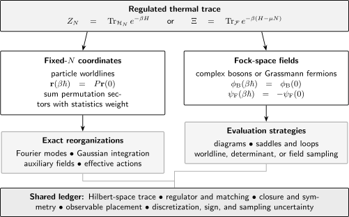
A thermal trace becomes a path integral only after a representation and finite-slice rule are chosen. Fixed-$N$ coordinates close up to permutations; bosonic and fermionic coherent fields obey periodic and antiperiodic thermal conditions. Transformations and approximations must preserve a shared ledger of regulator, symmetry, state, observable, and uncertainty.

Fields Replace Coordinates, Not Particles One for One

In a particle path integral, a configuration at one $\tau$ is the list

$$\big( \mathbf r_1(\tau), \ldots, \mathbf r_N(\tau) \big).$$

In a field path integral, a configuration at one $\tau$ is the whole spatial function

$$\mathbf x \longmapsto \psi(\mathbf x,\tau).$$

The field history is therefore

$$\psi: (\mathbf x,\tau) \longmapsto \psi(\mathbf x,\tau).$$

A single field configuration can contain support over many positions and many occupation sectors. It is not the path of one particle through spacetime.

On a spatial lattice with $L$ sites and $M$ time slices, a bosonic measure is an ordinary finite-dimensional integral,

$$\mathcal D\psi^* \mathcal D\psi \;\longleftrightarrow\; \prod_{j=0}^{M-1} \prod_{i=1}^{L} \frac{d\psi_{i,j}^*\,d\psi_{i,j}}{\pi}.$$

For fermions, each factor is a Berezin integral over Grassmann generators. The formal continuum measure means a declared limit of such regulated objects. There is no translation-invariant Lebesgue measure on an infinite-dimensional function space waiting to be used without definition.

Boundary Conditions Are Observable Data

Thermal closure follows from the trace and the transformation properties of the inserted object.

Coordinate paths

For distinguishable particles,

$$\mathbf r_a(\beta\hbar) = \mathbf r_a(0).$$

For identical particles,

$$\mathbf r_a(\beta\hbar) = \mathbf r_{P(a)}(0).$$

The permutation $P$ is summed with the appropriate statistics weight.

Microscopic coherent fields

Bosonic and fermionic fields obey

$$\begin{aligned} \phi(\tau+\beta\hbar) &= \phi(\tau), \\ \psi(\tau+\beta\hbar) &= -\psi(\tau). \end{aligned}$$

This produces the Matsubara grids

$$\begin{aligned} \nu_n &= \frac{2\pi n}{\beta\hbar}, \\ \omega_n &= \frac{(2n+1)\pi}{\beta\hbar}. \end{aligned}$$

Composite operators

Thermal parity follows the total fermion parity of the operator. A density

$$n = \psi^\dagger\psi$$

is bosonic and has periodic thermal correlators. A pair field

$$\Delta = \psi_\downarrow\psi_\uparrow$$

is also fermion-parity even, despite being built from fermions. A single fermion field is parity odd and uses the antiperiodic grid.

Twisted traces

A trace with an insertion,

$$Z_U = \operatorname{Tr} \left( Ue^{-\beta H} \right),$$

can produce a twisted closure. If $U$ acts as a phase rotation,

$$U\psi U^\dagger = e^{i\theta}\psi,$$

the endpoint relation acquires the corresponding phase in addition to the statistics sign. Flux insertion, symmetry-resolved traces, and imaginary chemical potentials are examples where the twist is physical data.

The Nonrelativistic Bose Field

For a regulated contact Bose gas, the Euclidean action is

$$\begin{aligned} S_{\mathrm B} &= \int_0^{\beta\hbar} d\tau \int d^d x\, \Bigg[ \hbar\psi^* \partial_\tau\psi \\ &\qquad+ \frac{\hbar^2}{2m} |\nabla\psi|^2 + (V-\mu)|\psi|^2 \\ &\qquad+ \frac{g_0}{2} |\psi|^4 \Bigg]. \end{aligned}$$

The field is periodic in $\tau$. The first-order derivative is the coherent state’s overlap term. It is not the positive kinetic energy $m\dot q^2/2$ of a coordinate path.

For a static homogeneous saddle,

$$\psi(\mathbf x,\tau) = \Phi_0,$$

stationarity gives

$$\left( -\mu + g_R|\Phi_0|^2 \right) \Phi_0 = 0.$$

The exact functional integral includes every field configuration. Retaining only $\Phi_0$ is a mean-field approximation. Gaussian fluctuations, topological configurations, and nonperturbative sampling are different evaluation strategies for the same regulated action.

The bare contact coupling $g_0$ must be matched using the same ultraviolet regulator used in the path integral. Replacing it by $4\pi\hbar^2a_s/m$ inside divergent loops without a matching prescription repeats the same error as in operator perturbation theory.

The Fermionic Field

For two fermion components,

$$\begin{aligned} S_{\mathrm F} &= \int_0^{\beta\hbar} d\tau \int d^d x\, \Bigg[ \sum_{\sigma} \bar\psi_\sigma \mathcal D_0 \psi_\sigma \\ &\qquad+ g_0\, \bar\psi_\uparrow \bar\psi_\downarrow \psi_\downarrow \psi_\uparrow \Bigg], \end{aligned}$$

where

$$\mathcal D_0 = \hbar\partial_\tau - \frac{\hbar^2\nabla^2}{2m} - \mu.$$

The Grassmann fields are antiperiodic. A same-component local $s$-wave monomial vanishes by antisymmetry; distinct spin components can interact in the displayed channel.

Grassmann integration is algebraic. For a quadratic matrix $M$,

$$\int \mathcal D\bar\psi \mathcal D\psi\, e^{-\bar\psi M\psi} \propto \det M.$$

The determinant is an ordinary number after the fermions are integrated out. It may be positive, negative, or complex, depending on symmetries, parameters, and the remaining fields.

From Lattice Hamiltonian to Spacetime Action

Consider the Hubbard model,

$$\begin{aligned} H &= -t \sum_{\langle ij\rangle,\sigma} \left( c_{i\sigma}^\dagger c_{j\sigma} + \mathrm{h.c.} \right) \\ &\quad+ U \sum_i n_{i\uparrow}n_{i\downarrow}. \end{aligned}$$

A coherent-state time lattice gives Grassmann variables $\psi_{i\sigma,j}$. The kinetic matrix contains:

• temporal nearest-neighbor differences;
• spatial hopping;
• chemical potential;
• antiperiodic closure on the last time link.

The local quartic interaction prevents direct Gaussian integration. One can introduce an auxiliary field through an exact Gaussian or discrete identity, provided the normalization, channel, and contour are stated. Schematically,

$$e^{-\epsilon_\tau U Q^2/\hbar} \propto \int d\phi\, \exp \left[ -A\phi^2 + B\phi Q \right].$$

After this transformation, the fermion action is quadratic:

$$\begin{aligned} \Xi &= \int\mathcal D\phi\, W_{\mathrm B}[\phi] \\ &\quad\times \det M_\uparrow[\phi]\, \det M_\downarrow[\phi]. \end{aligned}$$

The transformation can be exact at finite lattice spacing while Monte Carlo sampling, a saddle point, or truncation of the resulting bosonic action is approximate.

For the repulsive Hubbard model on a bipartite lattice at particle–hole-symmetric half filling, an appropriate decoupling can make the two spin determinants related so that their product is nonnegative. Doping, frustration, additional hopping, spin imbalance, or a different decoupling can remove that protection. “Fermionic” does not mean “always signed,” and “half-filled” does not mean “always sign free” without the full hypotheses.

Sources and Correlation Functions

Couple a source $J$ to an operator $\mathcal O$ by

$$S_{\mathrm E,J} = S_{\mathrm E} - \int_0^{\beta\hbar} d\tau \int d^d x\, J\mathcal O.$$

Define

$$Z[J] = \int\mathcal D\Phi\, e^{-S_{\mathrm E,J}/\hbar}.$$

Then

$$\frac{\delta\ln Z} {\delta J(x)} = \frac{1}{\hbar} \langle\mathcal O(x)\rangle_J.$$

The second derivative gives the connected correlator:

$$\begin{aligned} \frac{\delta^2\ln Z} {\delta J(x)\delta J(y)} &= \frac{1}{\hbar^2} \Big[ \langle\mathcal O(x)\mathcal O(y)\rangle_J \\ &\qquad- \langle\mathcal O(x)\rangle_J \langle\mathcal O(y)\rangle_J \Big]. \end{aligned}$$

Field insertions require the ordering and equal-time convention inherited from the finite time lattice. A fermionic two-point function is commonly

$$G(1,2) = -\left\langle \mathcal T_\tau \psi(1) \bar\psi(2) \right\rangle.$$

Its one-sided limits differ because of the canonical anticommutator. Replacing an adjacent-slice definition by a same-slice product without specifying the limit can lose contact terms.

Source derivatives generate imaginary-time observables. Real-frequency response requires spectral information and an analytic-continuation prescription; it does not follow by replacing $i\omega_n$ with $\omega+i0$ in arbitrary noisy data.

Perturbation Theory from the Path Integral

Split

$$\mathcal K = \mathcal K_0 + \mathcal V.$$

The interaction representation gives

$$\begin{aligned} \frac{Z}{Z_0} &= \left\langle \mathcal T_\tau \exp \left[ -\frac{1}{\hbar} \int_0^{\beta\hbar} d\tau\, \mathcal V_I(\tau) \right] \right\rangle_0. \end{aligned}$$

Expanding the exponential and applying Gaussian contractions produces Matsubara diagrams. In the functional language:

• the quadratic kernel gives propagator lines;
• interaction monomials give vertices;
• integrations impose spacetime or momentum-frequency conservation;
• Grassmann reordering gives fermion signs;
• $\ln Z$ keeps connected vacuum diagrams;
• source derivatives attach external operator insertions.

The path integral and operator Wick expansion are two organizations of the same perturbative series when their conventions match. A diagram is not an extra physical process added by the field representation.

Gaussian Integration and Effective Actions

Suppose fields are divided into retained variables $\phi$ and Gaussian variables $\chi$. Formally,

$$Z = \int\mathcal D\phi \mathcal D\chi\, e^{-S[\phi,\chi]/\hbar}.$$

Integrating out $\chi$ defines

$$e^{-S_{\mathrm{eff}}[\phi]/\hbar} \equiv \int\mathcal D\chi\, e^{-S[\phi,\chi]/\hbar}.$$

For bosonic Gaussian variables, the result contains an inverse determinant; for fermionic Gaussian variables, it contains a determinant. In logarithmic form,

$$\begin{aligned} S_{\mathrm{eff}}^{\mathrm B} &\supset +\frac{\hbar}{2} \operatorname{Tr}\ln A, \\ S_{\mathrm{eff}}^{\mathrm F} &\supset -\hbar \operatorname{Tr}\ln M, \end{aligned}$$

up to field reality, normalization, and multiplicity conventions.

Integrating out a field is exact if the functional integral is performed exactly. Expanding $\operatorname{Tr}\ln M$, making a derivative expansion, or keeping only selected modes introduces new approximations whose scale must be stated.

Gapless fields can generate nonlocal effective actions. A local polynomial ansatz is not guaranteed merely because the microscopic Hamiltonian was short ranged.

Saddle Points and Fluctuations

For an effective field $\phi$,

$$Z = \int\mathcal D\phi\, e^{-S_{\mathrm{eff}}[\phi]/\hbar}.$$

A saddle satisfies

$$\left. \frac{\delta S_{\mathrm{eff}}} {\delta\phi(x)} \right|_{\phi=\phi_*} = 0.$$

Writing

$$\phi = \phi_*+\delta\phi$$

gives

$$\begin{aligned} S_{\mathrm{eff}}[\phi] &= S_{\mathrm{eff}}[\phi_*] + \Delta S^{(2)} + \cdots, \\ \Delta S^{(2)} &= \frac12 \int dx\,dy\, \delta\phi(x) \\ &\qquad\times \Gamma^{(2)}(x,y) \delta\phi(y). \end{aligned}$$

The saddle is controlled when an explicit parameter suppresses fluctuations, such as large component number, weak coupling in the relevant channel, large occupation, high dimension, or a well-separated action scale. Large system size alone does not suppress every soft or critical mode.

At a continuous transition, the Hessian develops a small eigenvalue and a naive Gaussian expansion can fail. The path integral makes the failure visible but does not solve it automatically.

Monte Carlo Weights and the Sign Problem

After discretization and any exact algebraic transformations, suppose

$$Z = \sum_C W(C).$$

If $W(C)\ge0$, normalized weights can be sampled as probabilities. If the weight is signed or complex, write

$$W(C) = |W(C)|e^{i\theta(C)}.$$

Then

$$\langle A\rangle = \frac{ \left\langle A e^{i\theta} \right\rangle_{|W|} }{ \left\langle e^{i\theta} \right\rangle_{|W|} }.$$

The average phase is

$$\left\langle e^{i\theta} \right\rangle_{|W|} = \frac{Z}{Z_{|W|}}.$$

For an extensive system it often behaves as

$$\left\langle e^{i\theta} \right\rangle_{|W|} \sim \exp \left[ -\beta V \Delta f \right],$$

where $\Delta f$ is the appropriate free-energy-density difference. An exponentially small denominator produces exponentially poor signal to noise.

The sign problem depends on representation, basis, parameters, and algorithm. A change of variables can remove it in special cases. There is no generic efficient cure for all local fermionic models; the general problem contains NP-hard instances.

Absence of a sign problem does not imply that a simulation is easy. Critical slowing down, topological freezing, poor estimators, continuum extrapolation, and large autocorrelation times can remain.

The Sign Problem Preview derives the reweighted ratio, its free-energy and sample-cost scaling, the role of basis choice, and the limits of generic complexity claims.

Worldline, Determinant, and Field Algorithms

The path-integral representation suggests several numerical families.

Method family	Sampled object	Natural setting	Main diagnostics
path-integral Monte Carlo	coordinate worldlines and permutations	continuum bosons and distinguishable particles	time step, exchange updates, finite size
worldline or worm algorithms	occupation paths, loops, discontinuities	lattice bosons and selected spin models	ergodicity, winding sectors, autocorrelation
determinant quantum Monte Carlo	auxiliary fields with fermion determinants	interacting lattice fermions	determinant conditioning, sign, Trotter error
lattice field Monte Carlo	bosonic or effective fields	statistical and Euclidean field theories	cutoff, volume, critical slowing down
saddle and loop methods	stationary field plus fluctuations	controlled large-$N$, weak-coupling, or ordered regimes	Hessian spectrum and truncation order

The fictitious Monte Carlo trajectory through configurations is not real-time quantum evolution. It is an algorithm for sampling an equilibrium or Euclidean weight.

Imaginary Time Is Not Real Time

The Euclidean weight is

$$e^{-S_{\mathrm E}/\hbar}.$$

A real-time path integral has the oscillatory phase

$$e^{iS/\hbar}.$$

The two objects answer different questions. Equilibrium imaginary time is compact and tied to a trace. Real-time expectation values require initial state data and, for density operators, a forward-and-backward contour.

Analytic continuation is a statement about correlation functions with the required analyticity and spectral bounds. It is not a rule that maps sampled Euclidean field configurations one by one into physical real-time histories.

Real-Time Thermal Dynamics Preview develops the operator contour and nonequilibrium boundary data.

Toward Statistical Field Theory

Expand a periodic bosonic field in Matsubara modes:

$$\phi(\mathbf x,\tau) = \sum_{n\in\mathbb Z} \phi_n(\mathbf x) e^{-i\nu_n\tau}.$$

At sufficiently long distances near a thermal transition, nonzero modes can be heavy compared with the spatial scales of interest because

$$|\nu_n| \ge \frac{2\pi}{\beta\hbar} \qquad (n\ne0).$$

Integrating them out can leave a static effective functional for $\phi_0(\mathbf x)$:

$$Z \longrightarrow \int\mathcal D\phi_0\, e^{-\beta F_{\mathrm{eff}}[\phi_0]}.$$

This is dimensional reduction, not a universal identity at every temperature. It requires a bosonic zero mode, scale separation, and control of the operators generated by the removed modes. Fermionic fields have no zero Matsubara frequency and can still influence the coefficients and nonlocality of the remaining bosonic theory.

Landau–Ginzburg Theory Preview develops the static order-parameter functional. Statistical Field Theory Preview separates the resulting regulated field measure from the microscopic quantum path integral and distinguishes exact coarse-field weights from truncations.

Exact Steps and Approximate Steps

Step	Can be exact?	What must be declared
insert complete basis at finite $M$	yes	basis and trace
coherent-state resolution	yes	normalization, measure, and symbol
Trotter factorization at finite $\epsilon_\tau$	generally approximate	order and error scaling
sum permutation sectors	yes	statistics and internal states
Hubbard–Stratonovich identity	yes	channel, contour, constants
integrate a Gaussian field	yes	determinant and zero modes
continuum limit	yes when it exists	regulator and matching trajectory
saddle-point replacement	approximate	control parameter
truncate derivative or loop expansion	approximate	power counting and omitted order
Monte Carlo estimate	statistical approximation	autocorrelation and uncertainty
analytic continuation from noisy data	inverse problem	prior, covariance, and resolution

The word “path integral” names the representation, not the accuracy of every subsequent step.

Validation Workflow

For a reproducible many-body path-integral calculation:

1. Declare the trace. Canonical, grand canonical, projected, twisted, or real-time contour.
2. Declare the variables. Coordinates, coherent fields, local states, or auxiliary fields.
3. Fix the finite regulator. Spatial lattice or basis, time slices, volume, and boundary conditions.
4. Write the exact finite expression. Preserve adjacent-slice arguments and measure constants needed for free energies.
5. State the product formula. Include its order in $\epsilon_\tau$.
6. Track statistics. Permutation parity, Grassmann order, or determinant structure.
7. Match continuum couplings. Hold physical observables fixed as the ultraviolet cutoff changes.
8. Define observables on the lattice. State time placement, contact terms, and composite-operator renormalization.
9. Choose an evaluation method. Diagrammatic, saddle, worldline, determinant, or direct field sampling.
10. Converge every regulator. Time step, spatial cutoff, volume, bond decomposition, and numerical tolerances.
11. Measure conditioning. Average sign or phase, autocorrelation, effective sample size, and covariance.
12. Benchmark. Compare with a free limit, exact small system, sum rule, symmetry identity, or independent method.

Common Mistakes

1. Writing $\int\mathcal D\Phi$ without a regulator. The measure is defined by a finite construction and limiting prescription.
2. Calling every thermal path periodic. Identical-particle coordinates close up to permutations; fermionic coherent fields are antiperiodic.
3. Making fermion coordinates antiperiodic. This confuses worldline and coherent-state representations.
4. Treating a Grassmann field as a numerical stochastic field. Berezin integration is algebraic; ordinary sampling begins after Grassmann variables are integrated out.
5. Replacing operators by commuting fields before fixing ordering. Coherent-state actions use a specific finite-slice symbol.
6. Assuming a Euclidean weight is positive. Berry phases, fermion determinants, frustration, and chemical potentials can produce signs or phases.
7. Equating an exact decoupling identity with an exact saddle. The identity and its approximate evaluation are separate steps.
8. Ignoring determinant zeros and conditioning. A formally finite determinant can be numerically unstable.
9. Reading Monte Carlo time as physical time. It is a sampling coordinate.
10. Inferring real-time spectra directly from smooth imaginary-time data. Analytic continuation is ill conditioned.
11. Taking $M\to\infty$ but not the spatial continuum or thermodynamic limit. The limits address different errors.
12. Using a continuum contact coupling without matching. Bare couplings depend on the ultraviolet regulator.
13. Assuming all Hubbard decouplings have the same truncated saddle. Different channels can produce inequivalent approximations.
14. Treating a field redefinition as harmless for every observable. Composite operators and sources must transform too.
15. Reporting only statistical error. Trotter, volume, cutoff, fit, and autocorrelation errors may dominate.

Connections

• Imaginary Time supplies the operator semigroup and open-versus-closed distinction.
• Thermal Green Functions supplies ordered correlators and equal-time limits.
• Bosonic and Fermionic Matsubara Frequencies supplies the compact-time frequency grids.
• Coherent-State Path Integrals develops overlap-generated Berry geometry, first-order actions, and spin coherent fields.
• Diagrammatic Methods Preview develops line, vertex, symmetry-factor, and self-energy bookkeeping.
• Mean-Field Theory compares variational, factorization, and saddle constructions.
• Large-N and Saddle-Point Methods Preview supplies an explicit fluctuation-control parameter.
• Bose–Hubbard Model provides a worldline-friendly lattice boson example.
• Hubbard Model provides a determinant and auxiliary-field fermion example.
• Hubbard–Stratonovich Transformation Preview owns continuous and discrete identities, channel and contour choices, determinant weights, and the exact boundary before saddle approximations.
• Statistical Field Theory Preview develops regulated field measures, constrained coarse-field weights, generating functionals, and the boundary between saddles and fluctuations.
• Sources to Generating Functionals develops source differentiation and connected functionals.
• Euclidean Time to Euclidean QFT develops reflection positivity and Lorentzian reconstruction conditions.

References

1. M. Kac, “On Distributions of Certain Wiener Functionals”, Transactions of the American Mathematical Society 65, 1–13 (1949) – probabilistic foundation related to Euclidean coordinate paths.
2. R. P. Feynman, “Atomic Theory of the λ Transition in Helium”, Physical Review 91, 1291–1301 (1953) – permutation cycles and path-integral reasoning for quantum fluids.
3. H. F. Trotter, “On the Product of Semi-Groups of Operators”, Proceedings of the American Mathematical Society 10, 545–551 (1959) – product formula underlying time slicing.
4. M. Suzuki, “Generalized Trotter’s Formula and Systematic Approximants of Exponential Operators and Inner Derivations with Applications to Many-Body Problems”, Progress of Theoretical Physics 56, 1454–1469 (1976) – controlled higher-order product decompositions.
5. R. Blankenbecler, D. J. Scalapino, and R. L. Sugar, “Monte Carlo Calculations of Coupled Boson–Fermion Systems. I”, Physical Review D 24, 2278–2286 (1981) – integrating out fermions and sampling determinant-dependent bosonic fields.
6. D. Chandler and P. G. Wolynes, “Exploiting the Isomorphism between Quantum Theory and Classical Statistical Mechanics of Polyatomic Fluids”, Journal of Chemical Physics 74, 4078–4095 (1981) – ring-polymer representation and molecular applications.
7. J. E. Hirsch, “Discrete Hubbard–Stratonovich Transformation for Fermion Lattice Models”, Physical Review B 28, 4059–4061 (1983), with erratum in 29, 4159 – discrete auxiliary-field decoupling.
8. D. M. Ceperley, “Path Integrals in the Theory of Condensed Helium”, Reviews of Modern Physics 67, 279–355 (1995) – worldlines, permutation cycles, estimators, and path-integral Monte Carlo.
9. N. Prokof’ev, B. Svistunov, and I. Tupitsyn, “Worm Algorithm in Quantum Monte Carlo Simulations”, Physics Letters A 238, 253–257 (1998) – extended-configuration worldline sampling.
10. M. Troyer and U.-J. Wiese, “Computational Complexity and Fundamental Limitations to Fermionic Quantum Monte Carlo Simulations”, Physical Review Letters 94, 170201 (2005) – NP-hard instances of the generic sign problem.
11. J. W. Negele and H. Orland, Quantum Many-Particle Systems, CRC Press (2018 reissue) – coherent-state functional integrals and finite-temperature many-body methods.
12. A. Altland and B. Simons, Condensed Matter Field Theory, Cambridge University Press (2010) – field integrals, disorder and interaction decouplings, and effective actions.
13. J. H. Wilson and V. Galitski, “Breakdown of the Coherent State Path Integral: Two Simple Examples”, Physical Review Letters 106, 110401 (2011) – failures caused by naive continuum coherent-state prescriptions.

Exercises

1. Cyclic Trace in a Finite Basis

Let $\{|c\rangle\}$ be an orthonormal basis and set

$$T = e^{-\epsilon_\tau H/\hbar}.$$

For $M=3$, derive the complete basis sum for $Z_3=\operatorname{Tr}T^3$ and identify the cyclic boundary condition.

Solution

Start from

$$Z_3 = \sum_{c_0} \langle c_0|T^3|c_0\rangle.$$

Insert two identities:

$$I = \sum_{c_1}|c_1\rangle\langle c_1|, \qquad I = \sum_{c_2}|c_2\rangle\langle c_2|.$$

Then

$$\begin{aligned} Z_3 &= \sum_{c_0,c_1,c_2} \langle c_0|T|c_2\rangle \\ &\quad\times \langle c_2|T|c_1\rangle \langle c_1|T|c_0\rangle. \end{aligned}$$

With the uniform notation

$$\prod_{j=0}^{2} \langle c_{j+1}|T|c_j\rangle,$$

the trace requires

$$c_3 = c_0.$$

The cyclic closure comes from the trace, not from the Hamiltonian matrix elements themselves.

2. Classify Thermal Boundary Conditions

State the closure rule for:

1. one distinguishable particle coordinate;
2. $N$ identical boson coordinates;
3. a bosonic coherent field;
4. a fermionic coherent field;
5. a fermion density field.

Solution

For one distinguishable coordinate,

$$q(\beta\hbar) = q(0).$$

For identical boson coordinates,

$$\mathbf r_a(\beta\hbar) = \mathbf r_{P(a)}(0),$$

and all $P\in S_N$ are summed with positive weight.

A bosonic coherent field is periodic:

$$\phi(\beta\hbar) = \phi(0).$$

A fermionic coherent field is antiperiodic:

$$\psi(\beta\hbar) = -\psi(0).$$

The density $n=\bar\psi\psi$ is fermion-parity even, so its thermal correlators are periodic. The coordinate permutation rule and coherent-field antiperiodicity are two different implementations of statistics.

3. Two Ideal Identical Particles

Let

$$z_1(\beta) = \operatorname{Tr}_1 e^{-\beta h}$$

be the one-particle partition function. Show that

$$Z_2^{(\pm)} = \frac12 \left[ z_1(\beta)^2 \pm z_1(2\beta) \right].$$

Interpret the two terms as worldline sectors.

Solution

The two permutations are the identity $e$ and transposition $(12)$. Projection onto the symmetric or antisymmetric subspace gives

$$\begin{aligned} Z_2^{(\pm)} &= \frac12 \operatorname{Tr}_{1\otimes2} \left[ (I\pm P_{12}) e^{-\beta(h_1+h_2)} \right]. \end{aligned}$$

The identity term factorizes:

$$\operatorname{Tr} e^{-\beta(h_1+h_2)} = z_1(\beta)^2.$$

For the exchange term, choose one-particle eigenstates $|a\rangle$:

$$\begin{aligned} &\sum_{a,b} \langle a,b| P_{12} e^{-\beta(h_1+h_2)} |a,b\rangle \\ &\qquad= \sum_a e^{-2\beta\epsilon_a} = z_1(2\beta). \end{aligned}$$

The first contribution is two separately closed worldlines. The second is one exchange cycle of length $2\beta\hbar$, with positive sign for bosons and negative sign for fermions.

4. Dimensions of a Bosonic Euclidean Action

In $d$ spatial dimensions, verify that every term in

$$\begin{aligned} S_{\mathrm B} &= \int d\tau\,d^d x\, \Bigg[ \hbar\psi^*\partial_\tau\psi \\ &\qquad+ \frac{\hbar^2}{2m}|\nabla\psi|^2 + \frac{g}{2}|\psi|^4 \Bigg] \end{aligned}$$

has units of action when $[\psi]=L^{-d/2}$.

Solution

The measure has units

$$[d\tau\,d^d x] = T L^d.$$

For the temporal term,

$$\left[ \hbar\psi^*\partial_\tau\psi \right] = \frac{\hbar}{T L^d}.$$

Multiplying by the measure gives $\hbar$. For the gradient term,

$$\left[ \frac{\hbar^2}{m} |\nabla\psi|^2 \right] = \frac{E}{L^d},$$

so the measure again gives $ET$, the dimension of action.

Finally,

$$[g] = E L^d, \qquad [|\psi|^4] = L^{-2d}.$$

Thus $g|\psi|^4$ has units $E/L^d$, and its spacetime integral has units $ET=\hbar$.

5. Connected Correlator from Sources

Starting from

$$\begin{aligned} Z[J] &= \int\mathcal D\Phi\, e^{-S_J[\Phi]/\hbar}, \\ S_J[\Phi] &= S[\Phi] - \int dx\, J(x)\mathcal O(x), \end{aligned}$$

derive the first two derivatives of $\ln Z[J]$.

Solution

Differentiating once inserts $\mathcal O$:

$$\frac{\delta Z}{\delta J(x)} = \frac{Z[J]}{\hbar} \langle\mathcal O(x)\rangle_J.$$

Therefore

$$\frac{\delta\ln Z}{\delta J(x)} = \frac{1}{\hbar} \langle\mathcal O(x)\rangle_J.$$

Differentiating again acts both on the inserted operator average and on the normalization:

$$\begin{aligned} \frac{\delta^2\ln Z} {\delta J(x)\delta J(y)} &= \frac{1}{\hbar^2} \Big[ \langle\mathcal O(x)\mathcal O(y)\rangle_J \\ &\qquad- \langle\mathcal O(x)\rangle_J \langle\mathcal O(y)\rangle_J \Big]. \end{aligned}$$

The logarithm removes the disconnected product of one-point functions.

6. Bosonic Zero Mode

Let a periodic bosonic field have the expansion

$$\phi(\tau) = \sum_{n\in\mathbb Z} \phi_n e^{-i\nu_n\tau}.$$

Show that the time average isolates $\phi_0$. Explain why no analogous fermionic zero mode exists.

Solution

Orthogonality on the thermal circle gives

$$\int_0^{\beta\hbar} d\tau\, e^{-i\nu_n\tau} = \beta\hbar\,\delta_{n0}.$$

Hence

$$\frac{1}{\beta\hbar} \int_0^{\beta\hbar} d\tau\, \phi(\tau) = \phi_0.$$

Bosonic frequencies are

$$\nu_n = \frac{2\pi n}{\beta\hbar},$$

so $n=0$ is allowed. Fermionic frequencies are

$$\omega_n = \frac{(2n+1)\pi}{\beta\hbar},$$

which never vanish for integer $n$. Fermions can influence a static effective theory after being integrated out, but there is no elementary fermionic Matsubara zero mode.

7. Average Sign and Free-Energy Difference

Let

$$Z = \sum_C W(C), \qquad Z_{\mathrm{abs}} = \sum_C |W(C)|.$$

Show that the average sign in the absolute-weight ensemble is $Z/Z_{\mathrm{abs}}$. If

$$Z \sim e^{-\beta V f}, \qquad Z_{\mathrm{abs}} \sim e^{-\beta V f_{\mathrm{abs}}},$$

find its volume dependence.

Solution

Write

$$s(C) = \frac{W(C)}{|W(C)|}$$

where $W(C)\ne0$. Then

$$\begin{aligned} \langle s\rangle_{\mathrm{abs}} &= \frac{1}{Z_{\mathrm{abs}}} \sum_C |W(C)|s(C) \\ &= \frac{Z}{Z_{\mathrm{abs}}}. \end{aligned}$$

Using the extensive free energies,

$$\langle s\rangle_{\mathrm{abs}} \sim \exp \left[ -\beta V \left( f-f_{\mathrm{abs}} \right) \right].$$

Because $Z_{\mathrm{abs}}\ge|Z|$ in a real signed problem, $f-f_{\mathrm{abs}}\ge0$ in the thermodynamic limit under the usual conventions. A positive difference makes the average sign exponentially small in $\beta V$.

8. Audit an Auxiliary-Field Calculation

A calculation starts from a Hubbard Hamiltonian, applies a second-order Trotter formula, introduces an exact discrete auxiliary field, integrates out the fermions, and samples the field with Monte Carlo. Classify the exact and approximate steps, and list four independent convergence checks.

Solution

At a fixed spatial lattice and time step:

• inserting coherent-state identities is exact when the measure and symbol are correct;
• the discrete auxiliary-field identity is exact when its normalization and channel are retained;
• Gaussian Grassmann integration is exact and produces determinants;
• Monte Carlo averaging is an unbiased statistical estimator only after equilibration and in the absence of an uncontrolled sign reweighting failure.

The finite-step second-order Trotter factorization is approximate, with a global error that scales as the stated power of $\epsilon_\tau$. The final Monte Carlo estimate has statistical and autocorrelation uncertainty.

Independent checks include:

1. extrapolate $\epsilon_\tau\to0$;
2. increase spatial volume and control boundary conditions;
3. monitor the average sign and effective sample size;
4. increase warmup and sample length while binning beyond the autocorrelation time;
5. compare a small lattice with exact diagonalization;
6. verify particle–hole, spin, or sum-rule identities;
7. vary stabilization frequency and numerical precision for determinant products.

Agreement in only one of these limits does not establish the others.