Sign Problem Preview

A sign problem occurs when a chosen stochastic representation assigns negative or complex weights to configurations that one would like to sample as probabilities. The quantum partition function remains well defined. The obstruction is that large positive and negative, or differently phased, contributions cancel before producing the physical answer.

Suppose an exact representation gives

$$Z = \sum_C W(C),$$

with $W(C)\in\mathbb C$. Define

$$\begin{aligned} Z_{\mathrm{abs}} &= \sum_C |W(C)|, \\ \phi(C) &= \begin{cases} W(C)/|W(C)|, & W(C)\neq0, \\ 0, & W(C)=0. \end{cases} \end{aligned}$$

The absolute-weight ensemble is a valid probability distribution,

$$q_{\mathrm{abs}}(C) = \frac{|W(C)|}{Z_{\mathrm{abs}}},$$

but the desired partition function is recovered only after the phase is restored:

$$\left\langle\phi\right\rangle_{\mathrm{abs}} = \frac{Z}{Z_{\mathrm{abs}}}.$$

When this average sign or phase is exponentially small, ordinary sampling spends nearly all its effort estimating contributions that cancel.

Purpose and canonical scope

This page owns the many-body meaning and inferential consequences of sign and phase cancellations:

• how signed or complex weights arise from exchange, frustration, determinants, flux, and oscillatory actions;
• why reweighting converts cancellation into a small-denominator problem;
• why the required sample count can grow exponentially with inverse temperature and volume;
• why the presence and severity of the problem depend on basis, representation, parameters, and algorithm;
• which symmetry and positivity structures produce important sign-free cases;
• what exact cures, mitigations, and biased approximations do differently;
• what the standard complexity results establish and what they do not establish.

Monte Carlo Basics owns generic importance sampling and sample statistics. Quantum Monte Carlo Preview owns configuration spaces, updates, estimators, autocorrelation, and the full numerical evidence chain. Path Integrals for Many-Body Systems owns the functional-integral derivation, while Hubbard–Stratonovich Transformation Preview owns auxiliary-field identities and determinant construction.

The future Computational QM volume will own implementation-level reweighting workflows, stabilization, software tests, and benchmarks. Here the emphasis is the physical structure that makes a many-body representation easy or hard to sample.

Signed, complex, and vanishing weights

Three related cases should be distinguished.

A sign problem has real weights with

$$\phi(C) = \operatorname{sgn}W(C) \in \{-1,+1\}$$

for nonzero configurations.

A phase problem has genuinely complex weights,

$$\phi(C) = e^{i\theta(C)}.$$

A zero-overlap or rare-event problem can occur even with nonnegative weights when the sampling ensemble rarely visits configurations important to the target observable. It may produce similarly bad statistics, but it is not automatically a sign problem.

Negative and complex weights are not negative or complex probabilities. They are amplitudes, determinants, expansion coefficients, or effective-action factors whose sum yields a physical quantity. Sampling $|W|$ changes the theory being sampled; reweighting by $\phi$ is what restores the original one.

The exact reweighting identity

Let a configuration estimator $A(C)$ represent an observable. Then

$$\begin{aligned} \langle A\rangle &= \frac{ \sum_C W(C)A(C) }{ \sum_C W(C) } \\ &= \frac{ \left\langle \phi A \right\rangle_{\mathrm{abs}} }{ \left\langle \phi \right\rangle_{\mathrm{abs}} }. \end{aligned}$$

This identity is exact whenever the sums exist and $Z\neq0$. It does not say that the ratio is statistically well conditioned.

The numerator and denominator must be estimated from the same ensemble,

$$\begin{aligned} \widehat X &= \frac{1}{N} \sum_{t=1}^{N} \phi_t A_t, \\ \widehat Y &= \frac{1}{N} \sum_{t=1}^{N} \phi_t, \\ \widehat A &= \frac{\widehat X}{\widehat Y}. \end{aligned}$$

Their covariance matters. Reporting a small error bar for $\widehat X$ while treating $\widehat Y$ as exact can be dramatically misleading.

A two-configuration cancellation

Take

$$W(C_1) = 1, \qquad W(C_2) = -(1-\varepsilon),$$

with $0<\varepsilon\ll1$. Then

$$\begin{aligned} Z &= \varepsilon, \\ Z_{\mathrm{abs}} &= 2-\varepsilon, \\ \langle s\rangle_{\mathrm{abs}} &= \frac{\varepsilon}{2-\varepsilon}. \end{aligned}$$

Both sampled contributions are order one, while the desired residual is order $\varepsilon$. The difficulty is cancellation, not a small integrand.

Average sign as a free-energy ratio

For a thermal partition function of a Hermitian Hamiltonian, $Z>0$. Define

$$\begin{aligned} F &= -\frac{1}{\beta}\ln Z, \\ F_{\mathrm{abs}} &= -\frac{1}{\beta}\ln Z_{\mathrm{abs}}. \end{aligned}$$

Because $Z_{\mathrm{abs}}\ge Z$,

$$F \ge F_{\mathrm{abs}}.$$

The average phase is exactly

$$\left\langle\phi\right\rangle_{\mathrm{abs}} = \exp \left[ -\beta \left( F-F_{\mathrm{abs}} \right) \right].$$

For a volume $V$, write

$$F-F_{\mathrm{abs}} = V\Delta f_V.$$

Then

$$\left\langle\phi\right\rangle_{\mathrm{abs}} = e^{-\beta V\Delta f_V}.$$

If $\Delta f_V\to\Delta f>0$ as $V\to\infty$, the average phase falls exponentially in the space-time volume $\beta V$. This is not merely an empirical fitting form: $\Delta f_V$ is the finite-volume free-energy-density difference between the physical and absolute-weight ensembles.

The absolute ensemble is often called phase quenched, even in the real-sign case. It is generally a different statistical theory. Its dominant configurations need not resemble the configurations that survive after cancellation.

Why the sampling cost becomes exponential

For independent samples of $\phi$, let

$$\mu_\phi = \langle\phi\rangle_{\mathrm{abs}}.$$

Since $|\phi|=1$ on nonzero-weight configurations,

$$\mathbb E_{\mathrm{abs}} \left[ \left| \overline\phi-\mu_\phi \right|^2 \right] = \frac{ 1-|\mu_\phi|^2 }{ N }.$$

The relative root-mean-square uncertainty is therefore

$$\frac{ \sqrt{ \mathbb E \left| \overline\phi-\mu_\phi \right|^2 } }{ |\mu_\phi| } = \sqrt{ \frac{ 1-|\mu_\phi|^2 }{ N|\mu_\phi|^2 } }.$$

To resolve the denominator to relative precision $\epsilon$ requires approximately

$$N_{\mathrm{eff}} \gtrsim \frac{ 1-|\mu_\phi|^2 }{ \epsilon^2|\mu_\phi|^2 }.$$

When $|\mu_\phi|\ll1$,

$$N_{\mathrm{eff}} \gtrsim \epsilon^{-2} e^{2\beta V\Delta f_V}.$$

For a correlated Markov chain,

$$N_{\mathrm{eff}} \approx \frac{ N_{\mathrm{meas}} }{ 2\tau_{\mathrm{int},\phi} },$$

so autocorrelation multiplies an already exponential burden.

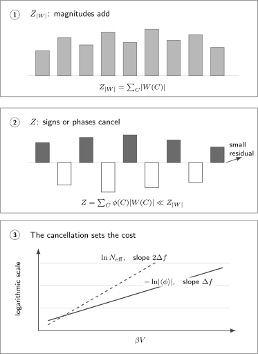
The absolute ensemble samples contributions that all add to $Z_{\mathrm{abs}}$. Restoring their signs or phases leaves the much smaller physical sum $Z$. If $|\langle\phi\rangle_{\mathrm{abs}}|\sim e^{-\beta V\Delta f}$, resolving that residual at fixed relative precision requires $N_{\mathrm{eff}}\sim e^{2\beta V\Delta f}$ effective samples.

Ratio uncertainty

Set

$$X = \phi A, \qquad Y = \phi, \qquad R = \frac{\mu_X}{\mu_Y}.$$

To first order,

$$\widehat R-R \approx \frac{ (\overline X-\mu_X) -R(\overline Y-\mu_Y) }{ \mu_Y }.$$

For independent samples, the corresponding mean-square error has the schematic form

$$\mathbb E \left| \widehat R-R \right|^2 \approx \frac{ \mathbb E_{\mathrm{abs}} \left| X-RY \right|^2 }{ N_{\mathrm{eff}}|\mu_Y|^2 }.$$

The same small denominator appears. For correlated chains, the numerator is replaced by an integrated autocovariance. Blocking, jackknife, or bootstrap analysis must preserve the joint numerator–denominator fluctuations.

The ratio estimator also has finite-sample bias. When $\widehat Y$ frequently approaches or crosses zero, a Gaussian error bar around $\widehat A$ is not trustworthy.

Where the cancellations come from

The sign problem is not synonymous with fermions, and fermions do not imply a sign problem in every formulation. Several mechanisms recur.

Fermion exchange in worldlines

For identical particles in a coordinate representation,

$$Z_N^{(\pm)} = \frac{1}{N!} \sum_P (\pm1)^P \int dR\, \rho(R,PR;\beta).$$

Bosonic exchange sectors add. Fermionic sectors carry the permutation parity $(-1)^P$. At low temperature, long exchange cycles can make even and odd sectors individually large while their difference remains small.

This is one origin of the fermion sign problem in path-integral Monte Carlo. It is not the only origin, and integrating out fermions can move the same cancellation into determinants rather than remove it.

Fermion determinants

After an auxiliary-field transformation, a common weight is

$$W[s] = W_{\mathrm B}[s]\, \det M_\uparrow[s]\, \det M_\downarrow[s].$$

The Grassmann integral producing each determinant is exact. The sampling problem begins when the determinant product is negative or complex across the ordinary auxiliary-field configurations.

At particle-hole-symmetric half filling, the repulsive one-band Hubbard Model on a bipartite lattice has a standard determinant-QMC formulation in which the spin determinants are related so that their product is nonnegative. Doping, frustrating hopping, magnetic flux, spin imbalance, or a different decoupling can destroy that relation.

Frustrated spins

Consider the transverse exchange of an antiferromagnetic Heisenberg model,

$$\begin{aligned} H_\perp &= \frac{J}{2} \sum_{\langle ij\rangle} \left( S_i^+S_j^- +S_i^-S_j^+ \right), \\ J &> 0. \end{aligned}$$

A local $\pi$ rotation about $z$ acts as

$$S_i^\pm \longmapsto \eta_i S_i^\pm, \qquad \eta_i\in\{-1,+1\}.$$

Every transverse bond becomes nonpositive if

$$\eta_i\eta_j = -1$$

on every antiferromagnetic edge. A bipartite graph permits this two-coloring. Around a triangle, however,

$$\begin{aligned} (\eta_1\eta_2) (\eta_2\eta_3) (\eta_3\eta_1) &= +1, \\ (-1)^3 &= -1. \end{aligned}$$

The requirements are inconsistent. The odd cycle carries a gauge-invariant obstruction to this simple sign rotation. This is how geometric frustration can generate signs even in a spin model with no mobile fermions.

Flux, Berry phases, and oscillatory actions

Complex hopping amplitudes may be written

$$t_{ij} = |t_{ij}|e^{iA_{ij}}.$$

Local phase redefinitions move $A_{ij}$ between bonds, but the loop phase

$$\Phi_\gamma = \sum_{(ij)\in\gamma} A_{ij} \pmod{2\pi}$$

is gauge invariant. A nontrivial flux can prevent all matrix elements from being made simultaneously real and nonpositive.

Berry-phase terms, finite-density fermion determinants, and real-time factors $e^{iS/\hbar}$ provide further complex-weight examples. Their detailed analytic structures differ, so one should not assume that a technique useful for one applies to all.

Stoquasticity and its limits

In a specified orthonormal basis $\{|x\rangle\}$, a real Hamiltonian is stoquastic if

$$\langle x|H|y\rangle \le 0 \qquad (x\neq y).$$

For small positive $\Delta\tau$,

$$\begin{aligned} \langle x| e^{-\Delta\tau H} |y\rangle &= \delta_{xy} \\ &\quad -\Delta\tau \langle x|H|y\rangle \\ &\quad +O(\Delta\tau^2). \end{aligned}$$

Nonpositive off-diagonal matrix elements therefore produce nonnegative leading short-time transitions. This supplies a broad route to sign-free worldline and stochastic-series formulations.

Three qualifications matter.

1. Stoquasticity is basis dependent.
2. Stoquasticity is sufficient for important QMC constructions, not a universal equivalence between Hamiltonians and all possible algorithms.
3. A sign-free representation can still be computationally difficult because of critical slowing down, topological freezing, poor overlap, ill-conditioned matrices, or hard-to-measure observables.

Quantum Annealing records whether a declared annealing Hamiltonian is stoquastic in a stated basis over the relevant time interval and owns only the process-level consequences. This page retains the definition, basis and representation dependence, sign-problem implications, and the warning that sign-free does not mean easy or advantageous.

Basis and representation dependence

The spectrum of a Hamiltonian does not determine the sign problem by itself. For example,

$$H = t\sigma^x, \qquad t>0,$$

has positive off-diagonal elements in the $\sigma^z$ basis. With $U=\sigma^z$,

$$UHU^\dagger = -t\sigma^x,$$

which is stoquastic in that basis. The physics is unchanged only if states and observables are transformed with the Hamiltonian.

This toy cure is local and obvious. In a many-body problem, a useful transformation must also be:

• computable without solving the original problem;
• compatible with locality or another tractable structure;
• accompanied by tractable transformed observables;
• effective over the parameter region of interest.

A formally sign-free basis that makes every operator exponentially nonlocal is not an efficient computational cure.

Representation dependence extends beyond basis rotations. Trotter decompositions, operator groupings, Hubbard–Stratonovich channels, fermion bags, loop decompositions, and partial analytic sums can assign different signs to their intermediate configurations while producing the same exact $Z$.

The average sign is therefore not a physical observable of $H$. It is a diagnostic of a specified representation and sampling measure.

Important sign-free structures

Sign-free cases arise from proofs, not from the hope that negative samples will be rare.

Structure	Positivity mechanism	Scope warning
unfrustrated bipartite spin model	a Marshall-type sublattice rotation makes transverse matrix elements nonpositive	additional frustrating bonds or phases can break the construction
spin-balanced attractive Hubbard formulation	the two real spin determinants coincide, giving a square	imbalance or altered couplings need separate analysis
repulsive bipartite Hubbard model at symmetric half filling	particle-hole symmetry relates the spin determinants	doping, frustrating hopping, flux, or another decoupling may restore signs
antiunitary determinant symmetry	eigenvalues or determinants occur in complex-conjugate pairs	the antiunitary action and its square must satisfy the theorem’s hypotheses
Majorana or reflection positivity	the fermionic weight factorizes or obeys a positivity cone	only specified interaction channels and decompositions qualify
meron or cluster regrouping	sign-canceling configurations are summed analytically before sampling	exact only for model and observable classes admitting the required cluster structure

Conjugate determinant pairing

A particularly transparent sufficient condition is

$$M_\downarrow[s] = M_\uparrow[s]^*.$$

Then

$$\begin{aligned} \det M_\downarrow[s] &= \left( \det M_\uparrow[s] \right)^*, \\ \det M_\uparrow[s]\, \det M_\downarrow[s] &= \left| \det M_\uparrow[s] \right|^2 \\ &\ge 0. \end{aligned}$$

More general antiunitary symmetries can enforce analogous conjugate pairing without a literal spin-up/spin-down factorization. The symmetry condition is formulation specific; time-reversal invariance of the physical Hamiltonian by itself is not enough unless it acts appropriately on every configuration matrix.

What counts as a cure?

The phrase “solve the sign problem” is too broad unless the method and guarantees are stated.

Exact transformations

An exact basis change, duality, auxiliary-field choice, or analytic regrouping can produce nonnegative weights while preserving the desired observable. This is a genuine cure for the stated model, parameter regime, and representation.

Meron-cluster and fermion-bag ideas can cancel families of signed configurations before stochastic sampling. They are powerful precisely because they exploit special algebraic structure; they are not black-box cures for arbitrary Hamiltonians.

Variance mitigation

A change of representation may increase the average sign without making it one. Better proposals, correlated sampling, control variates, and contour deformations may reduce variance. These can extend the reachable regime, but residual exponential scaling must still be measured.

Reweighting by $W/|W|$ is an exact identity, not a cure. It exposes the cancellation in a denominator.

Biased approximations

Fixed-node, constrained-path, phaseless, or related restrictions replace the uncontrolled cancellation with a condition informed by a trial state or path constraint. They can be extremely useful, but the constraint introduces bias unless an exactness theorem applies.

The result should be described as a constrained approximation and tested against released-constraint calculations, exact small systems, variational bounds when available, and trial-state dependence.

Analytic continuation from sign-free regions

Simulating at imaginary chemical potential, altered couplings, or another sign-free parameter and extrapolating to the target is a model-dependent inference problem. Its reliability depends on analyticity, truncation control, and proximity to singularities. A good fit does not by itself establish an exact cure.

The complexity result, stated carefully

Troyer and Wiese constructed a class of quantum systems for which a generic polynomial-time solution of the associated fermion sign problem would yield a polynomial-time solution of an NP-hard problem. Under the standard assumption that such problems do not all admit polynomial algorithms, no universal efficient cure should be expected.

This result does not prove that:

• every fermionic model is NP-hard;
• every negative weight is fatal at accessible sizes;
• every nonstoquastic Hamiltonian is hard;
• no special symmetry, duality, or regrouping can remove a particular sign problem;
• quantum Monte Carlo is inferior to every other method on sign-problem instances.

Related work shows that even finding a curing local basis transformation can be NP-complete for specified transformation classes. Again, this is a family-level worst-case statement. It does not replace model-specific analysis.

The useful conclusion is restrained: search energetically for structure in the problem at hand, but do not expect a representation-independent black-box algorithm that removes all sign problems efficiently.

Diagnosing severity in practice

A trustworthy study defines the diagnostic before presenting physics.

State the ensemble

Report the exact configuration weight $W(C)$, the sampled weight $|W(C)|$ or other proposal measure, and the phase factor used in reweighting. “We used QMC” is not enough.

Measure scaling, not one point

The average phase should be measured over a grid of:

• inverse temperatures $\beta$;
• spatial sizes and aspect ratios;
• densities, couplings, fluxes, and frustration parameters;
• boundary conditions;
• bases or decoupling channels being compared.

If exponential behavior is claimed, analyze

$$-\frac{ 1 }{ \beta V } \ln \left| \langle\phi\rangle_{\mathrm{abs}} \right|.$$

This quantity estimates $\Delta f_V$ only while the average phase is statistically resolved. Taking a logarithm of noise after the mean is consistent with zero creates a biased, meaningless plateau.

Resolve the denominator

An average sign should be quoted with an autocorrelation-aware uncertainty. A useful calculation requires more than a nonzero point estimate:

$$\frac{ |\widehat\mu_\phi| }{ \operatorname{SE}(\widehat\mu_\phi) } \gg 1.$$

The required significance depends on the observable ratio and the desired precision. Five standard errors in the denominator do not guarantee a precise nonlinear observable.

Preserve covariance

Store numerator and denominator in the same blocks. Apply jackknife or bootstrap resampling to the complete ratio, not to separately summarized error bars.

Benchmark the signed theory

At small size or high temperature, compare with exact diagonalization, direct enumeration, a series expansion, or a known sign-free limit. Agreement of the phase-quenched theory with itself is not a validation of the physical theory.

Test a claimed sign-free theorem

If symmetry predicts $W(C)\ge0$ configuration by configuration, inspect actual generated weights. A negative value then signals numerical roundoff, an inconsistent convention, or an implementation error rather than an unavoidable physical sign problem.

A compact evidence ledger

Claim	Minimum evidence	What the evidence does not establish
the formulation is sign free	configuration-level positivity proof plus numerical checks	rapid mixing or small total error
the sign problem is mild here	resolved average sign across the stated size and temperature window	favorable scaling outside that window
one basis is better	same physical observables, controlled transformations, and lower ratio variance	a universal optimum basis
a mitigation removes exponential cost	asymptotic scaling over increasing $\beta V$	exactness from a few small systems
a constrained method is accurate	release tests, exact benchmarks, and trial-state sensitivity	absence of bias in untested regimes
a complexity obstruction applies	an explicit reduction or theorem matching the model family	hardness of every individual instance

Common mistakes

• Calling a signed or complex weight a probability.
• Treating the phase-quenched ensemble as the original physical theory.
• Quoting numerator and denominator errors independently and ignoring covariance.
• Reporting $|\langle\phi\rangle|$ without an autocorrelation-aware uncertainty.
• Taking the logarithm of an unresolved average sign.
• Dropping negative configurations or replacing $W$ by $|W|$ without reweighting.
• Assuming all fermion models have a sign problem.
• Assuming bosonic or spin models are automatically sign free.
• Calling nonstoquasticity a proof that every QMC formulation fails.
• Treating the average sign as a basis-independent observable.
• Describing a constrained-path or fixed-node result as unbiased without a theorem.
• Citing NP-hardness as proof that one finite parameter point cannot be simulated.
• Concluding that sign-free sampling implies an easy or well-equilibrated calculation.

Exercises

Exercise 1: Cancellation and sample count

For the two weights

$$W_1 = 1, \qquad W_2 = -(1-\varepsilon),$$

find the absolute-ensemble probabilities, the average sign, and the leading effective sample count required to estimate the average sign with relative precision $\delta$ when $\varepsilon\ll1$.

Solution

The absolute partition function is

$$Z_{\mathrm{abs}} = 2-\varepsilon.$$

Therefore

$$\begin{aligned} q_1 &= \frac{1}{2-\varepsilon}, \\ q_2 &= \frac{1-\varepsilon}{2-\varepsilon}. \end{aligned}$$

The average sign is

$$\mu_s = q_1-q_2 = \frac{\varepsilon}{2-\varepsilon} \approx \frac{\varepsilon}{2}.$$

For $|\mu_s|\ll1$,

$$N_{\mathrm{eff}} \gtrsim \frac{1}{\delta^2\mu_s^2} \approx \frac{4}{\delta^2\varepsilon^2}.$$

The exact sum has only two terms, yet estimating their small difference by random sampling becomes quadratically expensive in $1/\varepsilon$.

Exercise 2: Free-energy cost

A phase-quenched simulation has

$$\beta V\Delta f_V = 5,$$

and $\tau_{\mathrm{int},\phi}=3$. Estimate the measurements needed to resolve the average phase to $10\%$ relative precision, using the small-phase approximation.

Solution

The average phase is

$$|\mu_\phi| = e^{-5}.$$

With $\epsilon=0.1$,

$$\begin{aligned} N_{\mathrm{eff}} &\gtrsim \epsilon^{-2} e^{10} \\ &\approx 100 \times 2.20\times10^4 \\ &\approx 2.2\times10^6. \end{aligned}$$

Autocorrelation gives

$$\begin{aligned} N_{\mathrm{meas}} &\approx 2\tau_{\mathrm{int},\phi} N_{\mathrm{eff}} \\ &\gtrsim 6 \times 2.2\times10^6 \\ &\approx 1.3\times10^7. \end{aligned}$$

This only resolves the denominator. A noisy observable numerator can require more samples.

Exercise 3: Why a triangle resists a sublattice cure

Let a local $z$ rotation assign $\eta_i=\pm1$ to each site and require $\eta_i\eta_j=-1$ on every antiferromagnetic bond. Prove that the condition is possible on every bipartite graph and impossible on an odd cycle.

Solution

On a bipartite graph, assign $\eta=+1$ on sublattice $A$ and $\eta=-1$ on sublattice $B$. Every edge joins opposite sublattices, so every product is $-1$.

For a cycle with vertices $1,\ldots,\ell$, multiply all bond conditions:

$$\prod_{i=1}^{\ell} \eta_i\eta_{i+1} = (-1)^\ell, \qquad \eta_{\ell+1} = \eta_1.$$

The left side is

$$\eta_1^2 \eta_2^2 \cdots \eta_\ell^2 = 1.$$

For odd $\ell$, the right side is $-1$, a contradiction. For even cycles, the alternating bipartite assignment is consistent.

Exercise 4: Determinant pairing

Suppose an auxiliary-field formulation obeys

$$M_2[s] = U M_1[s]^* U^{-1}$$

for every configuration $s$, with invertible $U$. Show that

$$\det M_1[s]\, \det M_2[s] \ge 0.$$

Solution

Similarity leaves the determinant unchanged:

$$\begin{aligned} \det M_2 &= \det \left( U M_1^* U^{-1} \right) \\ &= \det M_1^* \\ &= (\det M_1)^*. \end{aligned}$$

Hence

$$\begin{aligned} \det M_1\det M_2 &= |\det M_1|^2 \\ &\ge 0. \end{aligned}$$

The proof must hold configuration by configuration. Pairing only after averaging would not define a nonnegative sampling weight.

Exercise 5: Covariance in the reweighted ratio

Let $\widehat R=\overline X/\overline Y$ and $R=\mu_X/\mu_Y$. Derive the first-order fluctuation of $\widehat R$ and explain why strongly correlated numerator and denominator noise can reduce the ratio variance.

Solution

Write

$$\overline X = \mu_X+\delta X, \qquad \overline Y = \mu_Y+\delta Y.$$

Expanding the reciprocal,

$$\frac{1}{\mu_Y+\delta Y} \approx \frac{1}{\mu_Y} \left( 1-\frac{\delta Y}{\mu_Y} \right).$$

Therefore

$$\begin{aligned} \widehat R &\approx \frac{\mu_X}{\mu_Y} + \frac{\delta X}{\mu_Y} - \frac{\mu_X\delta Y}{\mu_Y^2} \\ &= R + \frac{ \delta X-R\delta Y }{ \mu_Y }. \end{aligned}$$

The variance depends on the combination $\delta X-R\delta Y$, which contains

$$-2\operatorname{Re} \left[ R^* \operatorname{Cov}(\delta X,\delta Y) \right].$$

Common fluctuations can cancel in the ratio. Separate error propagation discards this covariance and can overestimate or underestimate the uncertainty.

Exercise 6: Read the complexity claim

Classify each statement as supported or unsupported by the generic NP-hardness result.

1. No sign-problem-free formulation exists for any interacting fermion model.
2. A universal polynomial-time cure for the constructed family would have unlikely complexity consequences.
3. A particular doped Hubbard cluster is impossible to simulate accurately.
4. Special symmetries can remove signs without contradicting the worst-case theorem.

Solution

Statement 2 is supported: it captures the family-level worst-case result.

Statement 4 is also supported. A worst-case hardness theorem permits easy subclasses, special parameter points, and model-specific transformations.

Statements 1 and 3 are unsupported. Sign-free interacting fermion formulations are known, and a worst-case theorem does not decide the practical cost of one finite instance.

References

• J. E. Hirsch, “Two-Dimensional Hubbard Model: Numerical Simulation Study,” Physical Review B 31, 4403–4419 (1985). doi:10.1103/PhysRevB.31.4403
• E. Y. Loh Jr., J. E. Gubernatis, R. T. Scalettar, S. R. White, D. J. Scalapino, and R. L. Sugar, “Sign Problem in the Numerical Simulation of Many-Electron Systems,” Physical Review B 41, 9301–9307 (1990). doi:10.1103/PhysRevB.41.9301
• G. G. Batrouni and R. T. Scalettar, “Anomalous Decouplings and the Fermion Sign Problem,” Physical Review B 42, 2282–2289 (1990). doi:10.1103/PhysRevB.42.2282
• N. Hatano and M. Suzuki, “Representation Basis in Quantum Monte Carlo Calculations and the Negative-Sign Problem,” Physics Letters A 163, 246–249 (1992). doi:10.1016/0375-9601(92)91006-D
• D. M. Ceperley, “Path Integrals in the Theory of Condensed Helium,” Reviews of Modern Physics 67, 279–355 (1995). doi:10.1103/RevModPhys.67.279
• S. Chandrasekharan and U.-J. Wiese, “Meron-Cluster Solution of Fermion Sign Problems,” Physical Review Letters 83, 3116–3119 (1999). doi:10.1103/PhysRevLett.83.3116
• P. Henelius and A. W. Sandvik, “Sign Problem in Monte Carlo Simulations of Frustrated Quantum Spin Systems,” Physical Review B 62, 1102–1113 (2000). doi:10.1103/PhysRevB.62.1102
• M. Troyer and U.-J. Wiese, “Computational Complexity and Fundamental Limitations to Fermionic Quantum Monte Carlo Simulations,” Physical Review Letters 94, 170201 (2005). doi:10.1103/PhysRevLett.94.170201
• C. Wu and S.-C. Zhang, “Sufficient Condition for Absence of the Sign Problem in the Fermionic Quantum Monte Carlo Algorithm,” Physical Review B 71, 155115 (2005). doi:10.1103/PhysRevB.71.155115
• L. Wang, Y.-H. Liu, M. Iazzi, M. Troyer, and G. Harcos, “Split Orthogonal Group: A Guiding Principle for Sign-Problem-Free Fermionic Simulations,” Physical Review Letters 115, 250601 (2015). doi:10.1103/PhysRevLett.115.250601
• Z.-X. Li, Y.-F. Jiang, and H. Yao, “Solving the Fermion Sign Problem in Quantum Monte Carlo Simulations by Majorana Representation,” Physical Review B 91, 241117(R) (2015). doi:10.1103/PhysRevB.91.241117
• Z.-C. Wei, C. Wu, Y. Li, S. Zhang, and T. Xiang, “Majorana Positivity and the Fermion Sign Problem of Quantum Monte Carlo Simulations,” Physical Review Letters 116, 250601 (2016). doi:10.1103/PhysRevLett.116.250601
• Z.-X. Li, Y.-F. Jiang, and H. Yao, “Majorana-Time-Reversal Symmetries: A Fundamental Principle for Sign-Problem-Free Quantum Monte Carlo Simulations,” Physical Review Letters 117, 267002 (2016). doi:10.1103/PhysRevLett.117.267002
• V. I. Iglovikov, E. Khatami, and R. T. Scalettar, “Geometry Dependence of the Sign Problem in Quantum Monte Carlo Simulations,” Physical Review B 92, 045110 (2015). doi:10.1103/PhysRevB.92.045110
• M. Marvian, D. A. Lidar, and I. Hen, “On the Computational Complexity of Curing Non-Stoquastic Hamiltonians,” Nature Communications 10, 1571 (2019). doi:10.1038/s41467-019-09501-6
• Z.-X. Li and H. Yao, “Sign-Problem-Free Fermionic Quantum Monte Carlo: Developments and Applications,” Annual Review of Condensed Matter Physics 10, 337–356 (2019). doi:10.1146/annurev-conmatphys-033117-054307

Further study

• Quantum Monte Carlo Preview for configuration representations, estimators, autocorrelation, and validation.
• Monte Carlo Basics for generic importance sampling and effective sample size.
• Path Integrals for Many-Body Systems for permutation sectors and Euclidean field representations.
• Hubbard–Stratonovich Transformation Preview for determinant weights and decoupling dependence.
• Hubbard Model for the standard half-filled bipartite sign-free case and its limits.
• Heisenberg Model for bipartite and frustrated spin systems.
• Thermodynamic Potentials for the free-energy interpretation of the average phase.
• Validation Tests for independent computational evidence.