Exact Diagonalization Preview

Exact diagonalization, or ED, solves a declared finite many-body eigenproblem without introducing a physical approximation beyond the finite representation itself. One chooses a finite geometry, basis, local cutoff, boundary condition, and symmetry sector; represents the Hamiltonian on that space; computes all or selected eigenpairs; and evaluates observables from the resulting finite-system states.

The word exact is conditional:

$$\begin{gathered} \text{exact for the represented finite problem} \\ \neq \\ \text{exact for the thermodynamic system}. \end{gathered}$$

An eigensolver residual can be near machine precision while the physical result still has finite-size, boundary, cutoff, or model error. Conversely, a modest cluster can be uniquely valuable because it gives unbiased access to every state in the represented space, supplies sharp unit tests, and benchmarks methods that reach larger systems through additional approximations.

Purpose and Canonical Scope

This page owns the many-body construction and interpretation of finite diagonalization problems:

• basis enumeration for spins, fermions, and truncated bosons;
• matrix elements generated by local Hamiltonian terms;
• why local Hamiltonians are sparse in suitable bases;
• the distinction between a complete finite eigensystem and targeted sparse diagonalization;
• eigenstate, thermal, dynamical, and entanglement observables;
• exactness conditions, validation identities, and finite-size limitations;
• a two-spin Heisenberg example as a complete assembly and testing ledger.

Neighboring pages retain their canonical topics:

• Matrix Diagonalization owns dense numerical eigensolver concepts, residuals, stability, and degeneracy cautions.
• Sparse Matrices owns storage formats, sparse matrix-vector products, and matrix-free representations.
• Sparse Eigensolvers owns Krylov algorithms, targeting, restarting, and numerical convergence.
• Scaling of Hilbert Space owns exact basis counts and their asymptotics.
• Occupation-Number Representation owns the formal many-body basis language.
• Computational Many-Body Overview owns method selection, the full error ledger, and standards for qualified claims.
• Heisenberg Model owns the model physics used in the worked unit test.

Implementation-specific hashing, bit kernels, sparse libraries, parallel distribution, dense factorization choices, and performance benchmarks belong in Computational QM. This page develops enough structure to understand what an ED result means and how to test it.

Two Meanings of Exact Diagonalization

The literature uses ED in two related senses.

Complete diagonalization

A dense or structure-aware solver returns every eigenvalue and, when requested, a complete orthonormal eigenbasis:

$$H = \sum_{n=1}^{D} E_n |n\rangle \langle n|.$$

This form supports exact finite-temperature traces, arbitrary unitary evolution in the finite space, full level statistics, and complete Lehmann sums. Its memory cost is at least quadratic if a dense Hamiltonian or all eigenvectors are stored.

Targeted finite diagonalization

In many-body practice, ED can also mean constructing the exact finite Hamiltonian but using a sparse iterative solver to obtain only a few eigenpairs. The finite operator is still represented without a variational ansatz, but the output is incomplete:

$$\left\{ E_0,\ldots,E_{k-1} \right\}, \qquad k\ll D.$$

This route is appropriate for ground states and low excitations. It does not automatically provide a complete thermal trace or all spectral weight. Lanczos Method Preview explains the many-body workflow and evidence ledger; the general numerical recurrence remains canonical in Sparse Eigensolvers.

Whenever “ED” is reported, state which meaning is intended.

Declare the Finite Problem

A useful finite-problem record is

$$\mathcal F_L = \left( \Lambda_L, \mathcal B_L, \mathcal S_L, H_L, O_L \right).$$

Here:

• $\Lambda_L$ is the finite cluster and its geometry;
• $\mathcal B_L$ specifies boundary conditions;
• $\mathcal S_L$ is the represented basis or symmetry sector;
• $H_L$ is the finite Hamiltonian with all conventions fixed;
• $O_L$ denotes the observables to be evaluated.

The subscript $L$ is not decorative. A sequence of clusters can change shape, coordination, momentum grid, or boundary frustration as well as size. Boundary Conditions on Lattices explains why those choices are physical inputs.

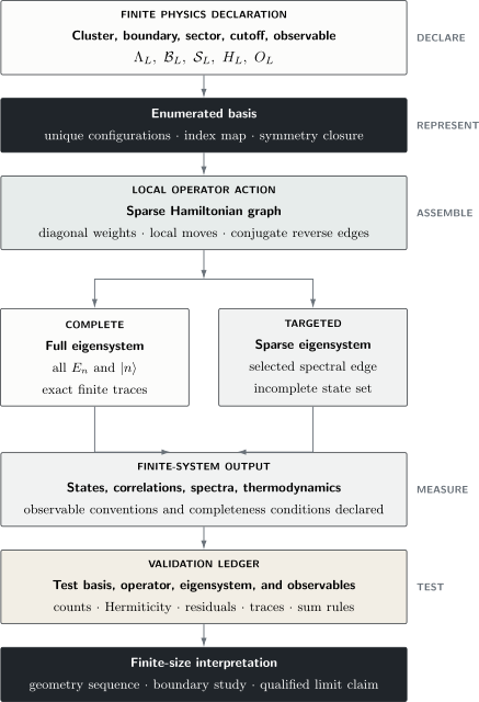
ED is exact only inside the declared finite space. Basis and operator tests establish the finite problem; solver tests establish the eigensystem; observable identities and a sequence of geometries determine how strongly the finite result supports a physical conclusion.

Constructing the Basis

Let

$$\mathcal S_L = \operatorname{span} \left\{ |a\rangle \right\}_{a=0}^{D-1}$$

be an orthonormal finite basis. A computational basis needs both a physical definition and an indexing convention:

$$|a\rangle \longleftrightarrow \text{configuration} \longleftrightarrow \text{integer index}.$$

The map must be one-to-one on the represented sector. Duplicate configurations, omitted states, or inconsistent ordering can produce a Hermitian matrix with the wrong physics, so basis validation precedes diagonalization.

Spin-one-half bitstrings

For $L$ spin-one-half sites, choose

$$b_i = \begin{cases} 1, & |\uparrow\rangle_i,\\ 0, & |\downarrow\rangle_i. \end{cases}$$

A product state is

$$|b_{L-1}\cdots b_1b_0\rangle,$$

and one possible integer encoding is

$$a = \sum_{i=0}^{L-1} b_i2^i.$$

The site-to-bit convention must be stated. Reversing endianness does not change a correctly transformed spectrum, but it changes every operator mask, basis label, and reshaping convention. A one-site product state is an inexpensive test of the convention.

The spin projection is

$$S_i^z |a\rangle = \hbar \left( b_i-\frac12 \right) |a\rangle.$$

If total $S^z$ is conserved, a fixed-$N_\uparrow$ sector contains only configurations satisfying

$$\sum_i b_i = N_\uparrow.$$

Its dimension is

$$D_{N_\uparrow} = \binom{L}{N_\uparrow}.$$

The counting derivation belongs to Scaling of Hilbert Space. Here the point is operational: the sector basis must contain exactly that many unique states, and every Hamiltonian action must remain inside it.

Fermionic occupation strings

For spinless fermionic modes ordered as $0,1,\ldots,M-1$, an occupation basis is

$$|\mathbf n\rangle = |n_{M-1}\cdots n_1n_0\rangle, \qquad n_i\in\{0,1\}.$$

The annihilation action includes the parity of occupied modes preceding $j$:

$$c_j|\mathbf n\rangle = (-1)^{p_j} n_j |\ldots,0_j,\ldots\rangle,$$

with

$$p_j = \sum_{i<j}n_i.$$

Changing the mode ordering changes intermediate signs and basis labels, although consistently transformed observables agree. A two-mode anticommutation test should be run before assembling an interacting Hamiltonian:

$$\left( c_i c_j^\dagger + c_j^\dagger c_i \right) |\mathbf n\rangle = \delta_{ij} |\mathbf n\rangle.$$

Fermionic Operators in Many-Body Models owns the operator algebra; ED turns that algebra into signed transitions between basis states.

Truncated bosonic occupations

Bosonic local spaces are infinite, so finite ED requires a declared truncation. A local cutoff uses

$$0 \leq n_i \leq n_{\max},$$

whereas a total-number cutoff uses

$$\sum_i n_i \leq N_{\max}.$$

These define different subspaces. The same symbol “cutoff 5” is meaningless without saying which rule is used. Observables sensitive to high occupation, such as onsite number variance, must be converged under cutoff enlargement.

The ladder factors

$$\begin{aligned} a_i|n_i\rangle &= \sqrt{n_i} |n_i-1\rangle, \\ a_i^\dagger|n_i\rangle &= \sqrt{n_i+1} |n_i+1\rangle \end{aligned}$$

must be combined with a boundary rule at $n_i=n_{\max}$. Silently discarding an attempted creation at the cutoff changes the represented operator and must be treated as truncation, not exact physics.

From Local Terms to a Sparse Hamiltonian

Write a local lattice Hamiltonian as

$$H = \sum_{X\subset\Lambda_L} h_X,$$

where each $h_X$ acts on a small set of sites or modes. Matrix elements are

$$H_{ab} = \langle a|H|b\rangle.$$

The useful computational object is often the action

$$H|b\rangle = \sum_a H_{ab}|a\rangle,$$

not a dense table of all $D^2$ possible entries. A local term changes only a few occupation labels, so each basis state connects to a small fraction of the full basis.

Define

$$\operatorname{nnz}(H) = \#\left\{ (a,b): H_{ab}\neq0 \right\}.$$

For many local models,

$$\operatorname{nnz}(H) \sim \operatorname{poly}(L)D,$$

even though $D$ itself grows exponentially. This makes sparse or matrix-free Hamiltonian application possible; it does not remove the exponential vector length.

Assembly as a configuration graph

It is useful to view the represented Hamiltonian as a weighted graph:

• basis states are vertices;
• diagonal terms give onsite vertex weights;
• off-diagonal terms connect configurations;
• matrix elements are edge weights;
• exact symmetries split the graph into disconnected components.

This picture exposes several tests. Every transition must land on a valid basis state. Reverse edges must carry conjugate amplitudes. A claimed conserved sector must be closed under every local term.

Hermiticity

For an orthonormal basis of a closed system,

$$H_{ab} = H_{ba}^\ast.$$

Common assembly errors include:

• adding a hopping or spin-flip transition in only one direction;
• double-counting an undirected bond;
• applying inconsistent complex phases on reverse links;
• using different basis-index conventions in diagonal and off-diagonal terms;
• forgetting a boundary bond or adding it twice.

Hermiticity is necessary but not sufficient. Two identically wrong off-diagonal entries can remain Hermitian.

Local Example: A Heisenberg Bond

For two spin-one-half sites,

$$H_{12} = J\, \mathbf S_1 \cdot \mathbf S_2.$$

Using dimensionless spin operators, $\mathbf S=\boldsymbol\sigma/2$, write

$$\mathbf S_1 \cdot \mathbf S_2 = S_1^zS_2^z + \frac12 \left( S_1^+S_2^- + S_1^-S_2^+ \right).$$

The local action is

$$\begin{aligned} \mathbf S_1\cdot\mathbf S_2 |\uparrow\uparrow\rangle &= \frac14 |\uparrow\uparrow\rangle, \\ \mathbf S_1\cdot\mathbf S_2 |\downarrow\downarrow\rangle &= \frac14 |\downarrow\downarrow\rangle, \end{aligned}$$

and

$$\begin{aligned} \mathbf S_1\cdot\mathbf S_2 |\uparrow\downarrow\rangle &= -\frac14 |\uparrow\downarrow\rangle + \frac12 |\downarrow\uparrow\rangle, \\ \mathbf S_1\cdot\mathbf S_2 |\downarrow\uparrow\rangle &= -\frac14 |\downarrow\uparrow\rangle + \frac12 |\uparrow\downarrow\rangle. \end{aligned}$$

These four rules are enough to assemble every Heisenberg bond in a product basis. The full Heisenberg Model page owns the model and its phases; here the bond is an operator-action template.

Complete Two-Spin Unit Test

Order the basis as

$$\left( |\uparrow\uparrow\rangle, |\uparrow\downarrow\rangle, |\downarrow\uparrow\rangle, |\downarrow\downarrow\rangle \right).$$

The matrix is

$$H_{12} = \frac{J}{4} \begin{pmatrix} 1 & 0 & 0 & 0\\ 0 & -1 & 2 & 0\\ 0 & 2 & -1 & 0\\ 0 & 0 & 0 & 1 \end{pmatrix}.$$

The parallel states are already eigenstates. The antiparallel block has symmetric and antisymmetric combinations:

$$\begin{aligned} |T_0\rangle &= \frac{ |\uparrow\downarrow\rangle + |\downarrow\uparrow\rangle }{\sqrt2}, & E_T &= \frac{J}{4}, \\ |S\rangle &= \frac{ |\uparrow\downarrow\rangle - |\downarrow\uparrow\rangle }{\sqrt2}, & E_S &= -\frac{3J}{4}. \end{aligned}$$

Together with $|\uparrow\uparrow\rangle$ and $|\downarrow\downarrow\rangle$, the symmetric states form a triplet at $J/4$ and the antisymmetric state is a singlet at $-3J/4$. Two Spin-One-Half Particles owns the angular-momentum derivation. ED recovers it from basis actions.

This tiny problem supports a strong unit-test suite:

$$\operatorname{Tr}H_{12} = 0,$$ $$\operatorname{Tr}H_{12}^2 = \frac{3J^2}{4},$$

and

$$\left[ H_{12}, S_1^z+S_2^z \right] = 0.$$

A many-site implementation should reproduce the same local matrix elements before any large sparse calculation is trusted.

Dense, Sparse, and Matrix-Free Representations

The represented operator and the eigensolver are separate choices.

Dense complete route

Storing a general complex dense Hamiltonian requires approximately

$$M_{\mathrm{dense}} \simeq 16D^2 \quad \text{bytes}$$

in complex double precision, before workspace and eigenvectors. A complete dense Hermitian eigensolve typically requires order-$D^3$ arithmetic, with algorithm-dependent constants and storage reductions.

This route is valuable when $D$ is small enough because completeness enables:

• every finite-system energy level;
• exact traces over the represented space;
• arbitrary operator matrices in the eigenbasis;
• full finite-system propagators;
• complete level and degeneracy audits.

Sparse stored route

A sparse representation stores nonzero values and their indices. Its memory scales with $\operatorname{nnz}(H)$ rather than $D^2$, plus indexing overhead. It is useful when the operator is reused for many matrix-vector products or several observables.

Sparse storage does not imply a sparse eigenvector. Generic interacting eigenstates can have nonzero amplitude on essentially every basis state.

Matrix-free route

A matrix-free implementation computes

$$|y\rangle = H|x\rangle$$

by applying local terms directly. It avoids storing the sparse matrix and can reduce memory, but it is harder to inspect. Tiny-system matrices, randomized Hermiticity checks, and exact action tests become especially important.

The formats and operation counts belong to Sparse Matrices.

Memory Is Usually the First Honest Estimate

A single complex state vector requires

$$M_{\mathrm{vec}} = 16D \quad \text{bytes}.$$

For an unconstrained $L=20$ spin-one-half system,

$$D = 2^{20} = 1{,}048{,}576.$$

Thus one vector is about $16$ MiB, while a dense complex matrix is about $16$ TiB:

$$\begin{aligned} M_{\mathrm{vec}} &\simeq 16\ \mathrm{MiB}, \\ M_{\mathrm{dense}} &\simeq 16\ \mathrm{TiB}. \end{aligned}$$

The fixed-$N_\uparrow=10$ sector has

$$D_{10} = \binom{20}{10} = 184{,}756.$$

One vector then needs about $2.82$ MiB, but a dense complex matrix still needs about $509$ GiB. Symmetry reduction can make sparse vector methods practical long after dense storage has failed.

Real calculations need several work vectors, basis-index data, sparse indices, observables, and solver workspace. Quoting only one-vector memory is a lower bound.

What a Complete Eigensystem Provides

Let

$$H|n\rangle = E_n|n\rangle, \qquad \langle m|n\rangle = \delta_{mn}.$$

Eigenstate observables

For an operator $O$,

$$\langle O\rangle_n = \langle n|O|n\rangle.$$

Off-diagonal matrix elements

$$O_{mn} = \langle m|O|n\rangle$$

control transitions, response, and dynamics. Operator conventions must match those used in the Hamiltonian basis.

Correlation functions

Equal-time correlations follow directly:

$$C_{ij}^{(n)} = \langle n| O_iO_j |n\rangle.$$

Connected correlations subtract one-point products. Their physical definitions and normalization choices belong to Connected Correlation Functions.

Exact finite-temperature traces

A complete spectrum gives

$$Z_L(\beta) = \sum_{n=1}^{D} e^{-\beta E_n},$$

and

$$\langle O\rangle_{\beta,L} = \frac{ \sum_n e^{-\beta E_n} \langle n|O|n\rangle }{ Z_L(\beta) }.$$

This is exact for the represented finite Hilbert space. It is not necessarily exact for an untruncated bosonic space or the thermodynamic system.

A low-energy subset can approximate low-temperature thermodynamics only when omitted weight is controlled. If $E_{\mathrm{cut}}$ is the first omitted energy, the suppression scale is

$$e^{-\beta \left( E_{\mathrm{cut}}-E_0 \right)},$$

but degeneracy and the number of omitted states also matter. “Low temperature” must be compared with both gaps and entropy.

Dynamical spectral sums

At zero temperature, a finite-system spectral measure for $O$ has the form

$$S_O(\omega) = \sum_n \left| \langle n|O|0\rangle \right|^2 \delta \left( \omega-\omega_{n0} \right),$$

where

$$\omega_{n0} = \frac{ E_n-E_0 }{\hbar}.$$

The exact finite result is a set of delta peaks. Any broadening used in a plot is an added resolution prescription. Spectral Functions owns the full definitions, conventions, and physical interpretation. Dynamical Correlation Functions Numerically shows how to benchmark this direct line list against Lanczos and real-time estimators with a matched kernel.

Entanglement from eigenvectors

For a bipartition $A\cup B$, reshape the coefficients as

$$|\psi\rangle = \sum_{a,b} C_{ab} |a\rangle_A |b\rangle_B.$$

Then

$$\rho_A = CC^\dagger.$$

The reshape depends on site ordering, bit convention, and subsystem choice. Product states and Bell pairs are essential tests. Entanglement Spectrum owns the full extraction and interpretation.

Degeneracy and Basis Dependence

Inside an exactly degenerate eigenspace, the solver may return any orthonormal basis. Individual vectors can rotate under tiny perturbations or changes of numerical library while the invariant subspace remains correct.

If $\mathcal D$ is a degenerate subspace, define its projector:

$$P_{\mathcal D} = \sum_{n\in\mathcal D} |n\rangle\langle n|.$$

The projector is basis independent. For a symmetry-resolved interpretation, diagonalize the commuting symmetry operator within $\mathcal D$ or construct the sector before solving. Do not infer broken symmetry from an arbitrary numerical combination of degenerate states.

Eigenvector phases are also arbitrary:

$$|n\rangle \longrightarrow e^{i\phi_n}|n\rangle.$$

Expectation values are unchanged, but raw vector components and off-diagonal phases are not. Regression tests should compare phase-invariant quantities or align phases by an explicit convention.

Validation Before Physics

A trustworthy ED calculation uses independent checks at several layers.

Basis checks

• expected state count and no duplicate indices;
• every configuration satisfies the declared constraints;
• index-to-state and state-to-index maps are inverses;
• simple product states have the expected local quantum numbers;
• every Hamiltonian transition lands in the represented sector.

Operator checks

• Hermiticity;
• commutation with claimed conserved quantities;
• exact local matrix elements;
• correct bond count and boundary terms;
• fermionic anticommutation and bosonic ladder factors;
• agreement between stored sparse and matrix-free actions on random vectors.

Eigensystem checks

For every normalized computed eigenpair,

$$|r_n\rangle = \left( H-E_n \right) |n\rangle.$$

Report absolute or scaled residuals and check

$$\langle m|n\rangle \simeq \delta_{mn}.$$

For a complete eigensystem,

$$\sum_n E_n = \operatorname{Tr}H,$$

and

$$\sum_n E_n^2 = \operatorname{Tr}H^2.$$

These identities detect missing eigenvalues, sector mismatches, and some assembly errors. Higher moments can be useful when independently available.

Observable checks

• exact sum rules;
• positive probabilities and nonnegative variances;
• known limits at zero coupling or decoupled sites;
• symmetry-forbidden matrix elements;
• derivative identities such as Hellmann–Feynman;
• agreement between direct time evolution and spectral reconstruction on tiny systems.

For a nondegenerate eigenstate,

$$\frac{dE_n}{d\lambda} = \left\langle n\left| \frac{\partial H} {\partial\lambda} \right|n\right\rangle.$$

This tests the Hamiltonian parameterization, state, observable, and finite-difference procedure together.

Cross-method checks

On overlapping sizes, compare:

• complete dense and sparse targeted eigenpairs;
• stored sparse and matrix-free operator actions;
• ED and MPS energies and correlations;
• ED and quantum Monte Carlo observables in sign-free regimes;
• analytic and numerical spectra in exactly solvable limits.

Agreement is strongest when the methods have different failure modes.

Small-System Limits

ED has a controlled finite-system exactness and an uncontrolled reach problem. Several cautions follow.

Discrete spectra are not continua

Finite systems have discrete energy levels. A dense cluster of peaks can approximate a continuum only with a declared joint limit in size and resolution.

Symmetry breaking is subtle

Finite eigenstates can preserve an exact symmetry even where the thermodynamic system breaks it. Order parameters may vanish while squared order parameters, structure factors, susceptibilities, or quasi-degenerate state families reveal ordering tendencies.

Shape can matter as much as site count

Two clusters with the same $L$ can have different shortest loops, aspect ratios, coordination defects, or momentum grids. A sequence chosen only by increasing $L$ can oscillate between incompatible geometries.

Boundary conditions can select sectors

Periodic, open, twisted, and antiperiodic boundaries change allowed momenta and finite-size corrections. Boundary averaging can reduce some shell effects but does not erase the need to report each boundary condition.

Accessible sizes can precede the asymptotic regime

A smooth trend over three clusters is not proof of asymptotic scaling. Finite-Size Effects owns the diagnosis of shape, shell, gap, boundary, and resolution mechanisms; Thermodynamic Limit owns the limiting target.

Finite-Size Use Without Overclaiming

Suppose ED produces $O_L$ on a cluster sequence. A qualified analysis distinguishes:

$$\begin{gathered} \text{finite-system fact}, \\ \text{trend across declared clusters}, \\ \text{thermodynamic inference}. \end{gathered}$$

The physical audit determines whether the leading mechanism is a boundary layer, quantized mode, shell, parity or shape subsequence, critical cutoff, or another effect. Finite-Size Scaling in Numerics then owns fit forms, competing correction structures, uncertainty, and robustness.

ED is particularly authoritative as:

• an exact finite-cluster statement;
• a local-operator and symmetry benchmark;
• a complete small-system spectral reference;
• a validation target for approximate methods;
• one controlled component of a broader finite-size argument.

It is least authoritative when a qualitative thermodynamic phase claim rests on one small cluster and one observable.

A Reproducible ED Record

Report:

• cluster coordinates, bond list, and boundary conditions;
• basis ordering, mode ordering, and local cutoffs;
• all symmetry sectors and quantum-number conventions;
• Hamiltonian normalization and constant energy shifts;
• dense, sparse, or matrix-free representation;
• whether the spectrum is complete or targeted;
• solver and arithmetic precision;
• residuals, orthogonality, and degeneracy tolerance;
• observable normalization and Fourier convention;
• raw finite-size data and any broadenings;
• exact limits, trace identities, and cross-method checks.

The Validation Tests page owns the reusable artifact standard. An ED dataset should be reproducible without reverse-engineering hidden basis or boundary conventions. Benchmark Problems supplies exact Ising, Heisenberg, Hubbard, and Bose–Hubbard finite-cluster contracts against which an implementation can be tested.

Common Mistakes

Calling the method exact without naming the space

State the finite geometry, sector, and cutoff. “Exact” never removes those declarations.

Forming a dense matrix by default

Local many-body Hamiltonians are usually sparse in a suitable basis. Estimate $D$, $D^2$, and $\operatorname{nnz}(H)$ before allocating.

Confusing a sparse Hamiltonian with a sparse state

Locality makes operator action sparse. It does not imply that interacting eigenvectors have few nonzero coefficients.

Mixing bit or mode orderings

Hamiltonian terms, observables, subsystem reshaping, and displayed basis labels must use the same convention.

Dropping fermionic parity signs

A hopping term can remain Hermitian while having the wrong many-fermion signs. Test anticommutation and tiny loops.

Double-counting bonds

If an undirected bond list contains both $(i,j)$ and $(j,i)$, a symmetric interaction can be doubled. Check coordination and total bond count.

Solving only one sector

The global ground state or first excitation can lie in another particle-number, magnetization, momentum, parity, or spin sector. Symmetry Sectors in Many-Body Numerics develops the compatible-label, orbit, block-reconstruction, and cross-sector checks needed to make that search complete.

Treating arbitrary degenerate eigenvectors as physical labels

Use projectors or diagonalize commuting observables inside the degenerate subspace.

Using a partial spectrum for an uncontrolled thermal trace

Low-energy states suffice only when omitted partition-function weight is bounded or demonstrably negligible.

Interpreting finite-size broadening as decay

A plotted linewidth set by $\eta$ is not a lifetime.

Comparing clusters only by site count

Shape, shortest loops, aspect ratio, and momentum resolution can dominate small-cluster behavior.

Exercises

1. Assemble the two-spin matrix

Starting from

$$\mathbf S_1\cdot\mathbf S_2 = S_1^zS_2^z + \frac12 \left( S_1^+S_2^- + S_1^-S_2^+ \right),$$

derive the $4\times4$ matrix in the ordered product basis used above.

Solution

The $S_1^zS_2^z$ term contributes $1/4$ to parallel states and $-1/4$ to antiparallel states. The ladder terms annihilate parallel states. On $|\uparrow\downarrow\rangle$, only $S_1^-S_2^+$ survives and produces $|\downarrow\uparrow\rangle$ with coefficient one; the prefactor gives $1/2$. The reverse action is identical.

Therefore

$$H_{12} = \frac{J}{4} \begin{pmatrix} 1 & 0 & 0 & 0\\ 0 & -1 & 2 & 0\\ 0 & 2 & -1 & 0\\ 0 & 0 & 0 & 1 \end{pmatrix}.$$

The matrix is Hermitian and block diagonal in total $S^z$.

2. Estimate memory before allocation

For an unconstrained $L=24$ spin-one-half system, estimate the memory for one complex double-precision vector and for a dense complex matrix. Use binary units.

Solution

The dimension is

$$D = 2^{24}.$$

At $16$ bytes per complex number,

$$M_{\mathrm{vec}} = 16\cdot2^{24} \ \text{bytes} = 256\ \text{MiB}.$$

The dense matrix requires

$$\begin{aligned} M_{\mathrm{dense}} &= 16 \left( 2^{24} \right)^2 \ \text{bytes} \\ &= 16\cdot2^{48} \ \text{bytes} \\ &= 4\ \text{PiB}. \end{aligned}$$

This excludes eigensolver workspace and eigenvector storage. Sparse or matrix-free action is mandatory, but even that still requires several $256$ MiB vectors.

3. Test a claimed conserved sector

A Hamiltonian is assembled in a fixed-$N_\uparrow$ spin basis. Give two independent numerical tests that the sector is closed.

Solution

First, apply every local Hamiltonian term to every basis state on a tiny system and verify that every nonzero output has the same $N_\uparrow$ and maps to a valid sector index.

Second, construct the number operator

$$N_\uparrow = \sum_i \left( S_i^z+\frac12 \right)$$

in the same convention and verify

$$\left[ H,N_\uparrow \right] = 0$$

to numerical precision. The transition-closure test exercises the basis map; the commutator test exercises the assembled matrices. Their failure modes differ.

4. Bound a partial thermal trace

Suppose all omitted states have energy at least $E_{\mathrm{cut}}$ and there are at most $R$ omitted states. Give an upper bound on their partition-function contribution.

Solution

Each omitted Boltzmann factor satisfies

$$e^{-\beta E_n} \leq e^{-\beta E_{\mathrm{cut}}}.$$

Therefore the omitted contribution obeys

$$Z_{\mathrm{omit}} \leq R e^{-\beta E_{\mathrm{cut}}}.$$

Relative to the ground-state contribution,

$$\frac{ Z_{\mathrm{omit}} }{ e^{-\beta E_0} } \leq R e^{-\beta \left( E_{\mathrm{cut}}-E_0 \right)}.$$

The factor $R$ shows why a gap alone is not enough: the number of omitted states can offset Boltzmann suppression.

5. Compare degenerate eigenspaces

Two diagonalization libraries return different orthonormal vectors for a twofold-degenerate eigenvalue. How should the results be compared?

Solution

Compare the projectors onto the degenerate subspaces:

$$P = |1\rangle\langle1| + |2\rangle\langle2|.$$

The individual vectors can be related by any $2\times2$ unitary rotation and arbitrary phases, so component-wise comparison is not meaningful. One can compare projector norms, principal angles between subspaces, traces of observables over the subspace, and symmetry-resolved vectors obtained by diagonalizing a commuting operator within it.

References

• H. Q. Lin, “Exact Diagonalization of Quantum-Spin Models,” Physical Review B 42, 6561–6567 (1990), doi:10.1103/PhysRevB.42.6561.
• C. Lanczos, “An Iteration Method for the Solution of the Eigenvalue Problem of Linear Differential and Integral Operators,” Journal of Research of the National Bureau of Standards 45, 255–282 (1950), doi:10.6028/jres.045.026.
• E. Dagotto, “Correlated Electrons in High-Temperature Superconductors,” Reviews of Modern Physics 66, 763–840 (1994), doi:10.1103/RevModPhys.66.763.
• A. W. Sandvik, “Computational Studies of Quantum Spin Systems,” in AIP Conference Proceedings 1297, 135–338 (2010), doi:10.1063/1.3518900.
• P. Weinberg and M. Bukov, “QuSpin: A Python Package for Dynamics and Exact Diagonalisation of Quantum Many Body Systems, Part I: Spin Chains,” SciPost Physics 2, 003 (2017), doi:10.21468/SciPostPhys.2.1.003.
• J. M. Zhang and R. X. Dong, “Exact Diagonalization: The Bose–Hubbard Model as an Example,” European Journal of Physics 31, 591–602 (2010), doi:10.1088/0143-0807/31/3/016.
• J. Jaklič and P. Prelovšek, “Finite-Temperature Properties of Doped Antiferromagnets,” Advances in Physics 49, 1–92 (2000), doi:10.1080/000187300243381.
• Y. Saad, Numerical Methods for Large Eigenvalue Problems, 2nd ed., SIAM, 2011, doi:10.1137/1.9781611970739.
• G. H. Golub and C. F. Van Loan, Matrix Computations, 4th ed., Johns Hopkins University Press, 2013.
• H. Fehske, R. Schneider, and A. Weiße, eds., Computational Many-Particle Physics, Springer, 2008, doi:10.1007/978-3-540-74686-7.

Further Study

• Computational Many-Body Overview
• Symmetry Sectors in Many-Body Numerics
• Lanczos Method Preview
• Dynamical Correlation Functions Numerically
• Benchmark Problems
• Scaling of Hilbert Space
• Occupation-Number Representation
• Number Operators and Conserved Quantities
• Boundary Conditions on Lattices
• Matrix Diagonalization
• Sparse Matrices
• Sparse Eigensolvers
• Spectral Functions
• Sum Rules
• Entanglement Spectrum
• Validation Tests