Occupation-Number Representation

The occupation-number representation describes a many-particle state by the population of each chosen one-particle mode. A basis vector has the form

$$\lvert \boldsymbol n\rangle = \lvert n_1,n_2,\ldots\rangle,$$

where $n_i$ counts particles in mode $i$. This replaces artificial particle-slot labels by physically meaningful mode populations.

For bosons,

$$n_i \in \{0,1,2,\ldots\},$$

whereas for fermions,

$$n_i \in \{0,1\}.$$

That compact difference carries Bose enhancement, Pauli exclusion, distinct Hilbert-space dimensions, and different operator signs.

The Many-Body Hilbert Spaces Overview explains when a fixed-number sector or Fock space is the appropriate model space. The foundational definitions of Fock space and number states live in Fock Space and Occupation Number and the Occupation-Number Basis. This page develops their many-body use: choosing a finite mode set, constructing symmetry sectors, translating fixed-$N$ wavefunctions, and building sparse Hamiltonian matrices.

Why Mode Occupations Are Natural

For identical particles, labels such as “particle 1” and “particle 2” are coordinate slots, not persistent physical identities. A first-quantized many-body wavefunction

$$\Psi(x_1,\ldots,x_N)$$

must therefore be symmetric for bosons or antisymmetric for fermions. Here $x$ may collect position, spin, and any other one-particle coordinate.

Occupation notation builds the exchange symmetry into the basis itself. Instead of listing all $N!$ permutations of mode assignments, it records only how many particles occupy each mode. This has three practical advantages:

• exchange symmetry is automatic;
• fixed-particle-number and other conserved sectors are easy to isolate;
• few-body operators connect only a small fraction of basis configurations.

The representation does not introduce new physics. It is a change of coordinates on the appropriate symmetric or antisymmetric many-particle Hilbert space.

Choose the Mode Basis First

Let the retained one-particle modes be an orthonormal set

$$\mathcal B_1 = \left\{ \lvert\varphi_1\rangle, \ldots, \lvert\varphi_M\rangle \right\}.$$

A mode can be a momentum and spin state, atomic spin-orbital, lattice-site orbital, trap eigenstate, Wannier orbital, or another one-particle basis state.

The occupation tuple

$$\boldsymbol n = (n_1,\ldots,n_M)$$

has meaning only relative to this ordered basis. In particular:

• a spin-up and spin-down orbital at the same site are different modes;
• two crystal momenta in the same band are different modes;
• a localized orbital and a momentum orbital belong to different mode bases;
• fermionic signs require a fixed ordering of the modes.

The sum

$$N(\boldsymbol n) = \sum_{i=1}^{M}n_i$$

is the total particle number of the configuration.

Fixed-N Sectors and Fock Space

A fixed-$N$ calculation retains only configurations satisfying

$$\sum_{i=1}^{M}n_i = N.$$

The corresponding sector is the symmetric or antisymmetric $N$-particle space built from the retained modes.

Fock space collects all allowed particle-number sectors:

$$\mathcal F_{\pm}(\mathcal h_M) = \bigoplus_N \mathcal H_N^{(\pm)}.$$

The plus sign denotes bosons and the minus sign denotes fermions. For $M$ fermionic modes, $N$ stops at $M$. For bosons, $N$ is unbounded unless a particle-number or local-occupation cutoff is imposed.

A number-conserving Hamiltonian can be diagonalized within one fixed-$N$ sector. Grand-canonical calculations and particle-nonconserving effective Hamiltonians require several sectors.

Constructing a Finite Many-Body Basis

A reliable basis construction follows a definite sequence.

1. Choose an ordered set of $M$ orthonormal one-particle modes.
2. Choose bosonic or fermionic statistics.
3. Specify the particle-number sector or sectors.
4. Impose any local occupation cutoff for bosons.
5. Impose compatible conserved quantum numbers, such as momentum or spin projection.
6. Enumerate every occupation tuple satisfying all constraints exactly once.
7. Assign a stable index to each tuple.

For a fixed-$N$ sector, write the configuration set as

$$\mathcal C_N = \left\{ \boldsymbol n: \sum_i n_i=N \right\},$$

with the statistical restrictions on $n_i$ understood.

A general pure state is then

$$\lvert\Psi_N\rangle = \sum_{\boldsymbol n\in\mathcal C_N} C_{\boldsymbol n} \lvert\boldsymbol n\rangle,$$

and normalization requires

$$\sum_{\boldsymbol n\in\mathcal C_N} \left\lvert C_{\boldsymbol n}\right\rvert^2 = 1.$$

Counting Bosonic Configurations

For $N$ identical bosons in $M$ modes without a local cutoff, the number of fixed-$N$ configurations is the stars-and-bars count

$$\begin{aligned} \dim\mathcal H_{N,M}^{(B)} &= \binom{N+M-1}{N} \\ &= \binom{N+M-1}{M-1}. \end{aligned}$$

The full bosonic Fock space over any nonzero finite mode set is infinite-dimensional because $N$ is unbounded.

If every mode is truncated to

$$0 \leq n_i \leq n_{\max},$$

then the unrestricted tensor-product basis has dimension

$$(n_{\max}+1)^M.$$

At fixed $N$, the dimension is instead the coefficient of $x^N$ in

$$\left( 1+x+\cdots+x^{n_{\max}} \right)^M.$$

The simple stars-and-bars formula applies only when the upper cutoff does not exclude any fixed-$N$ configuration.

Counting Fermionic Configurations

For $N$ identical fermions in $M$ complete one-particle modes,

$$\dim\mathcal H_{N,M}^{(F)} = \binom{M}{N}.$$

One chooses which $N$ modes are occupied. The full fermionic Fock space has dimension

$$\dim\mathcal F_F(\mathcal h_M) = 2^M.$$

The degeneracy label must already be included in $M$. For example, two lattice sites with spin up and spin down provide four fermionic modes, not two.

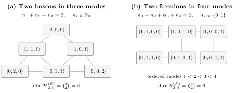
Fixed-$N$ occupation sectors. Two bosons distributed among three modes give six nonnegative-integer tuples. Two fermions distributed among four ordered modes also give six configurations, now represented by bitstrings with no repeated occupation.

Example: Two Bosons in Three Modes

For $N=2$ and $M=3$,

$$\dim\mathcal H_{2,3}^{(B)} = \binom{4}{2} = 6.$$

One convenient ordered basis is

$$\begin{aligned} \mathcal B_{2,3}^{(B)} = \bigl\{ &\lvert2,0,0\rangle, \lvert1,1,0\rangle, \lvert1,0,1\rangle, \\ &\lvert0,2,0\rangle, \lvert0,1,1\rangle, \lvert0,0,2\rangle \bigr\}. \end{aligned}$$

The tuple order is conventional, but it must remain fixed when state vectors and matrices are assembled.

Example: Two Fermions in Four Modes

For $N=2$ and $M=4$,

$$\dim\mathcal H_{2,4}^{(F)} = \binom{4}{2} = 6.$$

Using the mode order $1<2<3<4$, a basis is

$$\begin{aligned} \mathcal B_{2,4}^{(F)} = \bigl\{ &\lvert1,1,0,0\rangle, \lvert1,0,1,0\rangle, \lvert1,0,0,1\rangle, \\ &\lvert0,1,1,0\rangle, \lvert0,1,0,1\rangle, \lvert0,0,1,1\rangle \bigr\}. \end{aligned}$$

For a two-site spin-$1/2$ lattice model, one possible mode order is

$$(1\uparrow,1\downarrow,2\uparrow,2\downarrow).$$

In that convention, $\lvert1,1,0,0\rangle$ has double occupation of site $1$ by opposite spins, while $\lvert1,0,1,0\rangle$ has one spin-up fermion on each site.

A constrained basis may remove every tuple with $n_{i\uparrow}n_{i\downarrow}=1$ before any matrix is built. The t–J Model Preview develops this no-double-occupancy space and its projected hopping operators.

Normalized Basis States

The normalized bosonic number state is

$$\lvert n_1,\ldots,n_M\rangle_B = \prod_{i=1}^{M} \frac{ (b_i^\dagger)^{n_i} }{ \sqrt{n_i!} } \lvert0\rangle.$$

For fermions, fix the mode order and write

$$\lvert n_1,\ldots,n_M\rangle_F = (c_1^\dagger)^{n_1} \cdots (c_M^\dagger)^{n_M} \lvert0\rangle.$$

The factorial normalization and fermionic ordering conventions are developed canonically in Number States and Creation and Annihilation Operators. Here they establish an orthonormal many-body basis:

$$\langle\boldsymbol m\vert\boldsymbol n\rangle = \delta_{\boldsymbol m,\boldsymbol n}.$$

Translation from First Quantization

Choose orthonormal coordinate-space modes

$$\varphi_i(x) = \langle x\vert\varphi_i\rangle.$$

The fixed-$N$ occupation basis and the symmetric or antisymmetric first-quantized basis are unitarily equivalent.

Bosonic map

For an occupation tuple $\boldsymbol n$, form a list

$$I_{\boldsymbol n} = (i_1,\ldots,i_N)$$

in which mode label $r$ occurs $n_r$ times. The corresponding normalized symmetric wavefunction is

$$\begin{aligned} \Phi_{\boldsymbol n}^{(B)} &(x_1,\ldots,x_N) \\ &= \frac{1}{ \sqrt{ N!\prod_r n_r! } } \sum_{\pi\in S_N} \prod_{\alpha=1}^{N} \varphi_{i_\alpha} \left( x_{\pi(\alpha)} \right). \end{aligned}$$

Repeated mode labels make some permutation terms identical. The factor $\prod_r n_r!$ compensates for those repetitions.

Fermionic map

For a fermionic tuple, let

$$i_1 < i_2 < \cdots < i_N$$

be the occupied mode indices. The corresponding normalized antisymmetric wavefunction is the Slater determinant

$$\begin{aligned} \Phi_{\boldsymbol n}^{(F)} &(x_1,\ldots,x_N) = \frac{1}{\sqrt{N!}} \\ &\quad\times \det \left[ \varphi_{i_\alpha}(x_\beta) \right]_{\alpha,\beta=1}^{N}. \end{aligned}$$

The determinant vanishes if two complete one-particle modes coincide, which is the coordinate-space form of Pauli exclusion.

General fixed-N state

The coordinate wavefunction of

$$\lvert\Psi_N\rangle = \sum_{\boldsymbol n} C_{\boldsymbol n} \lvert\boldsymbol n\rangle$$

is

$$\Psi(x_1,\ldots,x_N) = \sum_{\boldsymbol n} C_{\boldsymbol n} \Phi_{\boldsymbol n}(x_1,\ldots,x_N).$$

Conversely,

$$C_{\boldsymbol n} = \langle\boldsymbol n\vert\Psi_N\rangle.$$

The amplitudes contain the same information as the symmetric or antisymmetric wavefunction after a complete mode basis has been chosen.

Worked Translation: Two in One Mode, One in Another

For three bosons with occupations

$$n_a=2, \qquad n_b=1,$$

the occupation vector $\lvert2_a,1_b\rangle_B$ corresponds to

$$\begin{aligned} \Phi_{2_a,1_b}^{(B)} ={}& \frac{1}{\sqrt3} \Bigl[ \varphi_a(x_1) \varphi_a(x_2) \varphi_b(x_3) \\ &+ \varphi_a(x_1) \varphi_b(x_2) \varphi_a(x_3) \\ &+ \varphi_b(x_1) \varphi_a(x_2) \varphi_a(x_3) \Bigr]. \end{aligned}$$

The three distinct assignments occur with equal amplitude. Orthogonality of $\varphi_a$ and $\varphi_b$ makes the three products mutually orthogonal, so the factor $1/\sqrt3$ normalizes the state.

Probabilities, Mean Occupations, and Coherence

For a pure state expanded in an orthonormal occupation basis,

$$p(\boldsymbol n) = \left\lvert C_{\boldsymbol n}\right\rvert^2$$

is the probability of obtaining the complete occupation pattern $\boldsymbol n$ in a projective measurement of all mode numbers.

The mean occupation of mode $i$ is

$$\langle N_i\rangle = \sum_{\boldsymbol n} \left\lvert C_{\boldsymbol n}\right\rvert^2 n_i.$$

Similarly,

$$\langle N_iN_j\rangle = \sum_{\boldsymbol n} \left\lvert C_{\boldsymbol n}\right\rvert^2 n_i n_j.$$

These diagonal observables depend only on occupation probabilities. Phase coherence between configurations matters for operators with off-diagonal matrix elements, such as hopping terms.

For a mixed state,

$$\rho = \sum_{\boldsymbol m,\boldsymbol n} \rho_{\boldsymbol m\boldsymbol n} \lvert\boldsymbol m\rangle \langle\boldsymbol n\rvert.$$

The diagonal entries are occupation probabilities. The off-diagonal entries are coherences in the chosen mode basis.

Hamiltonian Matrices in Occupation Space

An ideal diagonal one-body Hamiltonian has the form

$$H_0 = \sum_i \epsilon_i N_i.$$

Every occupation vector is an eigenstate:

$$H_0 \lvert\boldsymbol n\rangle = \left( \sum_i\epsilon_i n_i \right) \lvert\boldsymbol n\rangle.$$

This is why occupation numbers solve the ideal Bose and Fermi gases mode by mode.

A general one-body operator contains transfers between modes,

$$H_1 = \sum_{i,j} h_{ij} a_i^\dagger a_j.$$

Let $\boldsymbol e_i$ denote the unit occupation vector for mode $i$. For bosons and $i\neq j$,

$$\begin{aligned} b_i^\dagger b_j \lvert\boldsymbol n\rangle ={}& \sqrt{ (n_i+1)n_j } \\ &\times \lvert \boldsymbol n + \boldsymbol e_i - \boldsymbol e_j \rangle. \end{aligned}$$

The result is zero when $n_j=0$. Fermionic transfers obey the same occupation change when the source is occupied and the destination is empty, but acquire a sign fixed by mode ordering.

Two-body interactions connect configurations that differ by at most two occupied modes. Consequently, few-body Hamiltonians are usually sparse in a large occupation basis.

Worked Matrix: Two-Site Bosons

This section owns the finite-basis matrix benchmark. The model’s limits, phases, optical-lattice reduction, and diagnostics are developed in Bose–Hubbard Model.

Consider the two-site Bose–Hubbard Hamiltonian

$$\begin{aligned} H ={}& -J \left( b_1^\dagger b_2 + b_2^\dagger b_1 \right) \\ &+ \frac{U}{2} \sum_{i=1}^{2} N_i(N_i-1). \end{aligned}$$

In the fixed-$N=2$ basis

$$\mathcal B = \left( \lvert2,0\rangle, \lvert1,1\rangle, \lvert0,2\rangle \right),$$

the matrix is

$$[H]_{\mathcal B} = \begin{pmatrix} U & -\sqrt2J & 0 \\ -\sqrt2J & 0 & -\sqrt2J \\ 0 & -\sqrt2J & U \end{pmatrix}.$$

The interaction is diagonal. Hopping moves one boson and produces the factors $\sqrt2$. This three-state example already displays the general pattern used in exact diagonalization: enumerate configurations, apply each operator term, and accumulate sparse matrix elements.

Fermionic Signs and Ordered Modes

For ordered fermionic modes, define

$$Q_j(\boldsymbol n) = \sum_{i<j}n_i.$$

Then

$$\begin{aligned} c_j\lvert\boldsymbol n\rangle &= (-1)^{Q_j(\boldsymbol n)} n_j \lvert \boldsymbol n-\boldsymbol e_j \rangle, \\ c_j^\dagger\lvert\boldsymbol n\rangle &= (-1)^{Q_j(\boldsymbol n)} (1-n_j) \lvert \boldsymbol n+\boldsymbol e_j \rangle. \end{aligned}$$

The parity counts occupied modes crossed while bringing $c_j$ or $c_j^\dagger$ to its ordered position. Changing the mode order changes intermediate signs and basis phases, but not physical predictions when every operator and state is transformed consistently.

A fermionic bitstring is therefore more than a set of occupied labels: its ordered convention is part of the representation.

Basis Indexing in Computation

Numerical many-body calculations store a state as a coefficient vector indexed by configurations. Common encodings include:

• integer tuples for bosonic occupations;
• bitstrings for fermionic occupations;
• combinatorial ranks within a fixed-$N$ sector;
• symmetry-resolved tuples carrying momentum, spin projection, or parity.

For fermions, one possible bit-mask convention is

$$B(\boldsymbol n) = \sum_{i=1}^{M} n_i2^{i-1}.$$

This is an indexing convention, not a physical observable. Software must document whether mode $1$ is stored in the least-significant or most-significant bit and must use the same order for parity signs.

For bosons, a lookup table from occupation tuples to basis indices is often simpler than packing variable-width occupations into one integer.

Symmetry-Resolved Sectors

Particle number is only the first possible restriction. If a Hamiltonian conserves an additive quantum number

$$Q = \sum_i q_iN_i,$$

then each occupation vector has eigenvalue

$$Q(\boldsymbol n) = \sum_i q_i n_i.$$

One may retain only configurations with a chosen value of $Q$. Examples include:

• fixed spin projection $S_z$;
• fixed crystal momentum modulo a reciprocal lattice vector;
• fixed species populations;
• fixed parity or point-group sector after an appropriate basis construction.

If $[H,Q]=0$, different $Q$ sectors do not mix. Working within one block reduces memory use and prevents numerical eigenvectors from combining unrelated sectors.

Not every symmetry is diagonal in a chosen occupation basis. Spatial symmetries may require symmetry-adapted superpositions of occupation configurations rather than a simple tuple filter.

Mode Changes and Truncation

Let two orthonormal mode bases be related by a unitary matrix $U$:

$$d_\alpha^\dagger = \sum_i U_{i\alpha} a_i^\dagger.$$

A single occupation vector in the $a$ basis generally becomes a superposition of occupation vectors in the $d$ basis. Occupation is therefore basis-dependent even though the physical state is not.

With a complete one-particle basis, the transformation is exact. With a finite truncation, the basis choice affects convergence. Useful choices include:

• eigenmodes of the dominant one-body Hamiltonian;
• localized orbitals for short-range lattice interactions;
• natural orbitals adapted to the one-body density matrix;
• momentum modes when translation symmetry is central.

A compact basis is not automatically accurate. Convergence must be tested by increasing the mode set or occupation cutoff and monitoring the observables of interest.

Hilbert-Space Growth Remains Severe

Occupation notation removes redundant particle permutations, but it does not eliminate genuine many-body complexity.

For ten bosons in twenty modes,

$$\binom{29}{10} = 20{,}030{,}010$$

fixed-$N$ configurations remain. For twenty fermions in forty modes,

$$\binom{40}{20} = 137{,}846{,}528{,}820.$$

These dimensions explain why exact diagonalization requires modest systems, strong symmetry reduction, or both. Larger problems need approximation methods that exploit additional structure rather than merely a better label for the same exponentially large space.

Statistical Ensembles in This Representation

In an ideal gas whose Hamiltonian is diagonal in the selected modes, equilibrium probabilities factorize over occupation numbers in the grand-canonical ensemble. That special simplification underlies the Bose–Einstein and Fermi–Dirac distributions.

For an interacting Hamiltonian, an arbitrary occupation vector is generally not an energy eigenstate. The thermal density operator

$$\rho_\beta = \frac{e^{-\beta H}}{Z}$$

need not be diagonal in the occupation basis, even though that basis remains convenient for representing $H$ and $\rho_\beta$.

Likewise, a fixed mean occupation

$$\langle N_i\rangle$$

does not specify a unique many-body state. Many pure and mixed states can share the same one-mode averages while differing in fluctuations, coherences, and correlations.

Occupation Products and Entanglement

A single occupation vector is a product of mode-number states once a mode decomposition and ordering have been chosen. A superposition such as

$$\frac{1}{\sqrt2} \left( \lvert2,0\rangle + \lvert0,2\rangle \right)$$

can be entangled across the two mode algebras.

For fermions, the mode-factor description is a graded, order-dependent identification. It must not be treated as an ordinary tensor product of distinguishable particle subsystems; fermionic parity and the chosen observable algebras remain part of the physical statement.

For identical particles, statements about entanglement require a declared subsystem structure, operational algebra, and any relevant superselection restrictions. Particle labels should not be reintroduced as if they defined distinguishable subsystems.

Canonical Boundaries

This page owns:

• construction and counting of finite occupation bases for many-body models;
• fixed-$N$ bosonic and fermionic configuration sectors;
• the general translation to symmetric and antisymmetric coordinate wavefunctions;
• sparse Hamiltonian assembly in occupation space;
• computational indexing, symmetry reduction, and truncation cautions.

Other pages own:

• foundational Fock-space definitions: Fock Space and Occupation Number;
• basic occupation labels: Occupation-Number Basis;
• normalized number states: Number States;
• detailed mode-basis dependence: Mode Occupations;
• creation and annihilation algebra: Creation and Annihilation Operators;
• number operators and conservation criteria: Number Operators;
• general one- and two-body operator formulas: Many-Particle Hamiltonians.

Common Mistakes

• Treating occupation numbers as labels attached to identifiable particles.
• Writing an occupation tuple before declaring the mode basis and its order.
• Forgetting that spin-orbitals, not spatial orbitals alone, are fermionic modes.
• Using $\binom{N+M-1}{N}$ when a bosonic local cutoff removes configurations.
• Using $2^M$ for a fixed-$N$ fermionic sector instead of $\binom{M}{N}$.
• Omitting the factors $1/\sqrt{n_i!}$ from normalized bosonic number states.
• Ignoring the parity sign generated by ordered fermionic operators.
• Assuming a diagonal occupation operator makes the full interacting Hamiltonian diagonal.
• Confusing a basis product over modes with a statement about particle entanglement.
• Treating a finite mode truncation as exact without a convergence study.
• Enumerating configurations twice or changing their index order while assembling a matrix.

Exercises

Compare bosonic and fermionic sector sizes

For $N=3$ particles in $M=4$ modes, find the dimensions of the bosonic and fermionic fixed-$N$ sectors. List the fermionic configurations.

Solution

For bosons,

$$\dim\mathcal H_{3,4}^{(B)} = \binom{3+4-1}{3} = \binom{6}{3} = 20.$$

For fermions,

$$\dim\mathcal H_{3,4}^{(F)} = \binom{4}{3} = 4.$$

The fermionic bitstrings are

$$\begin{gathered} \lvert1,1,1,0\rangle, \quad \lvert1,1,0,1\rangle, \\ \lvert1,0,1,1\rangle, \quad \lvert0,1,1,1\rangle. \end{gathered}$$

Normalize a first-quantized bosonic state

Two orthonormal modes $a$ and $b$ contain three bosons with occupations $n_a=2$ and $n_b=1$. Derive the coordinate wavefunction and verify its normalization.

Solution

The distinct assignments of the $b$ mode to one of the three coordinate slots give

$$\begin{aligned} \Phi ={}& A \Bigl[ \varphi_a(x_1) \varphi_a(x_2) \varphi_b(x_3) \\ &+ \varphi_a(x_1) \varphi_b(x_2) \varphi_a(x_3) \\ &+ \varphi_b(x_1) \varphi_a(x_2) \varphi_a(x_3) \Bigr]. \end{aligned}$$

The three product functions are mutually orthogonal because $\langle\varphi_a\vert\varphi_b\rangle=0$. Therefore

$$1 = \langle\Phi\vert\Phi\rangle = 3\lvert A\rvert^2.$$

Choosing the overall phase real and positive gives

$$A = \frac{1}{\sqrt3}.$$

This agrees with the general normalization factor after repeated permutations are combined.

Add a site-energy bias

Add

$$H_\Delta = \frac{\Delta}{2} (N_1-N_2)$$

to the two-site, two-boson Hamiltonian. Find the matrix in the ordered basis $(\lvert2,0\rangle,\lvert1,1\rangle,\lvert0,2\rangle)$.

Solution

The bias eigenvalues are $\Delta$, $0$, and $-\Delta$ on the three basis states. It does not change the hopping matrix elements. Thus

$$\begin{gathered} [H+H_\Delta]_{\mathcal B} \\ = \begin{pmatrix} U+\Delta & -\sqrt2J & 0 \\ -\sqrt2J & 0 & -\sqrt2J \\ 0 & -\sqrt2J & U-\Delta \end{pmatrix}. \end{gathered}$$

The bias breaks the site-exchange symmetry unless $\Delta=0$.

Compute occupation fluctuations

For two bosonic modes, consider

$$\lvert\Psi\rangle = \frac{1}{2}\lvert2,0\rangle + \frac{1}{\sqrt2}\lvert1,1\rangle + \frac{1}{2}\lvert0,2\rangle.$$

Find $\langle N_1\rangle$, $\operatorname{Var}(N_1)$, and $\operatorname{Cov}(N_1,N_2)$.

Solution

The configuration probabilities are $1/4$, $1/2$, and $1/4$. Therefore

$$\langle N_1\rangle = \frac14(2) + \frac12(1) + \frac14(0) = 1.$$

Also,

$$\langle N_1^2\rangle = \frac14(4) + \frac12(1) = \frac32,$$

so

$$\operatorname{Var}(N_1) = \frac32-1 = \frac12.$$

By symmetry, $\langle N_2\rangle=1$. Only $\lvert1,1\rangle$ contributes to $N_1N_2$, giving

$$\langle N_1N_2\rangle = \frac12.$$

Hence

$$\operatorname{Cov}(N_1,N_2) = \frac12-1 = -\frac12.$$

The negative covariance ensures zero fluctuation of the fixed total $N_1+N_2=2$.

Track a fermionic parity sign

Use the ordered modes $1<2<3<4$ and the state

$$\lvert1,0,1,1\rangle = c_1^\dagger c_3^\dagger c_4^\dagger \lvert0\rangle.$$

Evaluate $c_2^\dagger\lvert1,0,1,1\rangle$ and $c_3\lvert1,0,1,1\rangle$.

Solution

For $c_2^\dagger$, one occupied mode lies to the left:

$$Q_2 = n_1 = 1.$$

Mode $2$ is empty, so creation is allowed and

$$c_2^\dagger \lvert1,0,1,1\rangle = -\lvert1,1,1,1\rangle.$$

For $c_3$, the occupations to the left are $n_1=1$ and $n_2=0$, so

$$Q_3 = 1.$$

Mode $3$ is occupied, and therefore

$$c_3 \lvert1,0,1,1\rangle = -\lvert1,0,0,1\rangle.$$

Both minus signs follow from the declared mode ordering.

Cross-Links

• Occupation-Number Basis
• Number States
• Mode Occupations
• Bosonic Fock Space
• Fermionic Fock Space
• Creation and Annihilation Operators
• Number Operators
• One-Body Operators
• One-Body Operators in Many-Body Models
• Two-Body Operators
• Two-Body Operators in Many-Body Models
• Many-Particle Hamiltonians
• Field Operators in Many-Body Models
• Tight-Binding Model
• Hubbard Model
• Scaling of Hilbert Space
• Quantum Statistics Overview
• Ideal Bose Gas
• Ideal Fermi Gas
• Reference Bridge: Fock Space

References

• A. L. Fetter and J. D. Walecka, Quantum Theory of Many-Particle Systems, Dover (2003).
• J. W. Negele and H. Orland, Quantum Many-Particle Systems, Westview Press (1998).
• H. Bruus and K. Flensberg, Many-Body Quantum Theory in Condensed Matter Physics, Oxford University Press (2004).
• A. Altland and B. Simons, Condensed Matter Field Theory, 2nd ed., Cambridge University Press (2010).
• P. Coleman, Introduction to Many-Body Physics, Cambridge University Press (2015).
• G. D. Mahan, Many-Particle Physics, 3rd ed., Springer (2000).
• A. Szabo and N. S. Ostlund, Modern Quantum Chemistry, Dover (1996).
• E. Dagotto, “Correlated electrons in high-temperature superconductors,” Reviews of Modern Physics 66, 763–840 (1994).