First-Quantized Many-Body Wavefunctions

A first-quantized many-body wavefunction is the coordinate representation of a fixed-particle-number quantum state. For $N$ particles it has the form

$$\Psi(q_1,\ldots,q_N,t) = \langle q_1,\ldots,q_N\vert\Psi(t)\rangle,$$

where each complete one-particle label $q_i$ may include position, spin, species-internal labels, band indices, or other retained degrees of freedom. If only position is present, one often writes

$$\Psi(\mathbf r_1,\ldots,\mathbf r_N,t).$$

The wavefunction is not a collection of $N$ one-particle waves. It is generally one complex amplitude on a $dN$-dimensional configuration space. Its dependence on all coordinates carries exchange structure and correlations that cannot, in general, be assigned to individual particles.

This page owns the use of coordinate wavefunctions in many-body models: configuration space, internal labels, normalization, fixed-$N$ Hamiltonians, observables, species bookkeeping, and translation to Fock-space language. The Symmetrization Postulate and Symmetric and Antisymmetric Wavefunctions own the foundational exchange rule and explicit orbital constructions. Occupation-Number Representation owns practical mode-basis construction.

“First quantization” names a representation of ordinary quantum mechanics. It does not mean that the particles follow classical trajectories or that second quantization is a different physical theory.

Coordinate Amplitudes

Let the one-particle Hilbert space be

$$\mathcal h = L^2(\Omega,d^dr) \otimes \mathbb C^{g},$$

where $\Omega$ is the spatial domain and $g$ counts retained discrete internal states. Write

$$q=(\mathbf r,\sigma,a,\ldots)$$

for the complete coordinate, with $\sigma$ a spin label and $a$ any additional internal index. It is convenient to define

$$\int dq\,f(q) \equiv \sum_{\sigma,a,\ldots} \int_\Omega d^dr\, f(\mathbf r,\sigma,a,\ldots).$$

Then a normalized pure fixed-$N$ state satisfies

$$\int dq_1\cdots dq_N\, \left| \Psi(q_1,\ldots,q_N) \right|^2 = 1.$$

The shorthand

$$dq^N \equiv dq_1\cdots dq_N$$

will be used below. Coordinate kets are distribution-normalized in continuous variables, so $\Psi$ is a square-integrable amplitude rather than an ordinary component in a finite orthonormal basis.

A mixed state does not have one wavefunction. It is represented by a density operator with coordinate kernel

$$\rho(q_1,\ldots,q_N;q_1',\ldots,q_N').$$

Writing a thermal or incoherent mixed state as a single $\Psi$ discards physical information.

Configuration Space

For $N$ particles moving in a region $\Omega\subseteq\mathbb R^d$, the ordered coordinate space is

$$\mathcal Q_N^{\mathrm{ord}} = \Omega^N.$$

A point

$$Q = (\mathbf r_1,\ldots,\mathbf r_N)$$

specifies one simultaneous configuration. It is not a list of trajectories. The time-dependent wavefunction assigns an amplitude to every such configuration at each time.

The dimension $dN$ is already a major many-body difficulty. Ten particles in three dimensions require a wavefunction on a 30-dimensional space before spin is included. Discretizing each one-particle coordinate with $M$ basis functions produces up to $M^N$ slot coefficients before exchange symmetry is used.

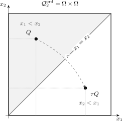
For two spinless particles in one spatial dimension, the ordered configuration space is the square $\Omega\times\Omega$. Exchange reflects $Q=(x_1,x_2)$ across the coincidence diagonal $x_1=x_2$ to $\tau Q=(x_2,x_1)$. Identical-particle wavefunctions obey $\Psi(\tau Q)=\eta\Psi(Q)$, with $\eta=+1$ for bosons and $\eta=-1$ for fermions, while the probability density is the same at the reflected points. One triangular region can represent unordered configurations only after its measure, diagonal, and boundary conditions have been specified.

Boundaries and excluded configurations

The domain is part of the Hamiltonian problem. A box may impose Dirichlet, Neumann, periodic, twisted, or other boundary conditions. A hard-core model can exclude the coincidence set

$$\Delta = \left\{ Q: \mathbf r_i=\mathbf r_j \text{ for some }i\ne j \right\}.$$

Singular interactions can instead leave the diagonal in the coordinate space while imposing short-distance boundary conditions on the operator domain. Removing a set and forcing the wavefunction to vanish there are related in some models but are not universally the same mathematical construction.

Ordered cover and physical configurations

For identical particles, slot labels are a convenient coordinate cover. The corresponding unordered spatial configurations are represented schematically by

$$\mathcal Q_N^{\mathrm{unord}} = \Omega^N/S_N,$$

or by

$$(\Omega^N\setminus\Delta)/S_N$$

when coincidences are excluded. In standard three-dimensional nonrelativistic quantum mechanics, one usually works on the ordered cover and imposes bosonic or fermionic exchange symmetry. This keeps differential operators and integrals simple.

The quotient viewpoint becomes important when topology matters. In two dimensions, exchanges are classified by braids rather than only permutations, allowing statistics beyond the boson and fermion cases. That extension is not assumed on this page.

Distinguishable Particles

For genuinely distinguishable particles, the one-particle spaces may differ:

$$\mathcal H_N = \mathcal h_1 \otimes\cdots\otimes \mathcal h_N.$$

The coordinate wavefunction is

$$\Psi(q_1,\ldots,q_N) = \langle q_1\vert\otimes\cdots\otimes \langle q_N\vert\Psi\rangle.$$

Here slot $i$ refers to a physically addressable subsystem or species. No symmetry condition relates $q_i$ and $q_j$ unless the model has an additional symmetry that does so.

For example, an electron and a nucleus have different masses, charges, and internal spaces. Exchanging their coordinate arguments does not describe exchange of identical particles. Their wavefunction may still be entangled:

$$\Psi(\mathbf r_e,\mathbf R_n) \ne \psi_e(\mathbf r_e) \chi_n(\mathbf R_n).$$

Distinguishability therefore does not imply factorization.

Several Identical Species

Many-body models often contain several species with fixed populations

$$N_1,N_2,\ldots,N_s.$$

The coordinate wavefunction may be organized as

$$\Psi( q_{1,1},\ldots,q_{1,N_1}; q_{2,1},\ldots,q_{2,N_2}; \ldots ).$$

Exchange symmetry is imposed within each identical species. If species $a$ is fermionic, then exchanging $q_{a,i}$ and $q_{a,j}$ changes the sign. No such requirement exchanges an electron coordinate with a proton coordinate.

Two internal states of one atom can be treated in more than one way. If coherent dynamics converts the states into each other, it is often best to regard the internal label as part of one complete coordinate $q=(\mathbf r,\sigma)$. If two stable components are modeled as separately conserved species, separate coordinate lists can be convenient. The Hamiltonian and allowed observables determine which organization is appropriate.

Spinor-Valued Wavefunctions

For spin-$1/2$ particles, a coordinate wavefunction has components

$$\Psi_{\sigma_1\cdots\sigma_N} (\mathbf r_1,\ldots,\mathbf r_N), \qquad \sigma_i\in\{\uparrow,\downarrow\}.$$

Normalization means

$$\sum_{\sigma_1,\ldots,\sigma_N} \int d^dr_1\cdots d^dr_N\, \left| \Psi_{\sigma_1\cdots\sigma_N} (\mathbf r_1,\ldots,\mathbf r_N) \right|^2 = 1.$$

If spin is not measured, the spatial probability density is obtained by summing the component probabilities:

$$p(\mathbf r_1,\ldots,\mathbf r_N) = \sum_{\sigma_1,\ldots,\sigma_N} \left| \Psi_{\sigma_1\cdots\sigma_N} (\mathbf r_1,\ldots,\mathbf r_N) \right|^2.$$

One must not sum amplitudes over unresolved orthogonal spin outcomes. The alternatives are exclusive measurement outcomes, so their probabilities add.

Spin-dependent operators act as matrices on these components. For example,

$$\mathbf S_i = \frac{\hbar}{2} \boldsymbol\sigma_i$$

acts on the $i$th spin index while leaving the coordinate arguments unchanged.

Exchange Acts on Complete Labels

For identical bosons or fermions, exchanging slots $i$ and $j$ gives

$$\Psi(\ldots,q_i,\ldots,q_j,\ldots) = \eta \Psi(\ldots,q_j,\ldots,q_i,\ldots),$$

where

$$\eta = \begin{cases} +1, & \text{bosons},\\ -1, & \text{fermions}. \end{cases}$$

More generally,

$$\Psi(q_{\pi(1)},\ldots,q_{\pi(N)}) = \eta(\pi) \Psi(q_1,\ldots,q_N),$$

with $\eta(\pi)=1$ for bosons and $\eta(\pi)=\operatorname{sgn}(\pi)$ for fermions.

The complete label must be exchanged. For particles with spin,

$$q_i = (\mathbf r_i,\sigma_i),$$

so exchange sends

$$(\mathbf r_i,\sigma_i) \longleftrightarrow (\mathbf r_j,\sigma_j).$$

Antisymmetrizing only the spatial arguments while leaving spin labels attached to slots generally gives the wrong total state. The canonical spin-spatial bookkeeping is developed in Spin and Spatial Wavefunctions.

Because $|\eta|=1$,

$$\left| \Psi(q_{\pi(1)},\ldots,q_{\pi(N)}) \right|^2 = \left| \Psi(q_1,\ldots,q_N) \right|^2.$$

Bosons and fermions therefore have permutation-invariant configuration probabilities. Their distinction survives in phases and signs, which affect interference, nodes, spectra, and operator matrix elements.

Slot Labels Are Not Particle Names

The notation $q_1,ldots,q_N$ does not assign persistent identities to identical particles. Slot $1$ tells the wavefunction which argument is being integrated, differentiated, or permuted. It does not identify a detectable particle that remains “particle 1” through time.

For an identical-particle observable, all slots must be treated consistently. A physical one-body operator has the form

$$A^{(1)} = \sum_{i=1}^{N} a(i),$$

not simply $a(1)$, unless $a(1)$ is being used as an intermediate device inside a permutation-symmetric expression.

Labeling a coordinate axis is unavoidable. Assigning that label an observable individuality is the mistake.

Probability on Ordered Coordinates

For distinguishable particles, the probability of finding $q_i$ in regions $A_i$ is

$$P(A_1,\ldots,A_N) = \int_{A_1}dq_1\cdots \int_{A_N}dq_N\, |\Psi(q_1,\ldots,q_N)|^2.$$

For identical particles, measurable events should not refer to an unobservable slot identity. Suppose two particles are spinless and $A$ and $B$ are disjoint spatial regions. The event “one particle is in $A$ and one is in $B$” is the union of two slot assignments:

$$\begin{aligned} P_{A,B} &= \int_A dx_1 \int_B dx_2\, |\Psi(x_1,x_2)|^2 \\ &\quad+ \int_B dx_1 \int_A dx_2\, |\Psi(x_1,x_2)|^2. \end{aligned}$$

Permutation invariance of $|\Psi|^2$ makes the two terms equal, so

$$P_{A,B} = 2 \int_A dx_1 \int_B dx_2\, |\Psi(x_1,x_2)|^2.$$

There is no universal instruction to divide every identical-particle integral by $N!$. Such factors depend on whether one integrates over the ordered cover, an unordered quotient, or a restricted fundamental region and on how the measure is defined.

One-Particle Number Density

For normalized identical-particle $\Psi$, define the one-particle number density in complete-coordinate notation by

$$n(q) = N \int dq_2\cdots dq_N\, |\Psi(q,q_2,\ldots,q_N)|^2.$$

It integrates to particle number:

$$\int dq\,n(q) = N.$$

If spin is unresolved, the spatial density is

$$n(\mathbf r) = \sum_\sigma n(\mathbf r,\sigma).$$

The probability density for the coordinate of a randomly selected particle is $n(q)/N$. Confusing this normalized marginal with the number density produces missing factors of $N$.

The same quantity is the expectation value of the first-quantized density operator

$$\hat n(q) = \sum_{i=1}^{N} \delta(q-q_i),$$

where the delta symbol includes Kronecker deltas for discrete internal labels.

Pair Density

The ordered pair density is

$$\begin{aligned} n^{(2)}(q,q') &= N(N-1) \int dq_3\cdots dq_N \\ &\quad\times |\Psi(q,q',q_3,\ldots,q_N)|^2. \end{aligned}$$

Its normalization is

$$\int dq\,dq'\, n^{(2)}(q,q') = N(N-1).$$

This convention counts ordered distinct pairs. An unordered-pair convention carries a factor $1/2$. Declaring the convention matters whenever pair correlations or interaction energies are compared across sources.

Time Evolution

The many-body Schrödinger equation is

$$i\hbar \frac{\partial}{\partial t} \Psi(q_1,\ldots,q_N,t) = H \Psi(q_1,\ldots,q_N,t).$$

For particles with masses $m_i$, external one-body terms $U_i$, and pair interactions $V_{ij}$, a common Hamiltonian is

$$H = \sum_{i=1}^{N} \left[ -\frac{\hbar^2}{2m_i}\nabla_i^2 +U_i(q_i) \right] + \sum_{i<j} V_{ij}(q_i,q_j).$$

Spin-orbit coupling, magnetic fields, nonlocal potentials, and other internal interactions make $U_i$ or $V_{ij}$ matrix-valued in the discrete indices. The coordinate equation then couples spinor components.

Pair-counting conventions

The two forms

$$\sum_{i<j}V(i,j)$$

and

$$\frac12 \sum_{i\ne j}V(i,j)$$

are equal when

$$V(i,j)=V(j,i).$$

The factor $1/2$ removes the double counting of ordered pairs. It is not an exchange-statistics factor.

Operator domains matter

The differential expression does not by itself define the Hamiltonian. One must also specify its Hilbert space, boundary conditions, and operator domain. Coulomb singularities, zero-range interactions, hard cores, and inverse-square potentials require particular care.

A formal wavefunction that is square-integrable but violates the Hamiltonian domain may not be an admissible state for the stated problem. Likewise, integrating by parts to prove Hermiticity is valid only when the boundary terms vanish under the chosen conditions.

Exchange-Invariant Dynamics

For identical particles, the Hamiltonian must commute with slot permutations:

$$U(\pi)HU(\pi)^\dagger = H.$$

Equivalently,

$$[H,U(\pi)] = 0.$$

Then a bosonic or fermionic initial state remains in the same exchange sector:

$$\begin{aligned} U(\pi)\lvert\Psi(t)\rangle &= U(\pi)e^{-iHt/\hbar} \lvert\Psi(0)\rangle \\ &= e^{-iHt/\hbar}U(\pi) \lvert\Psi(0)\rangle \\ &= \eta(\pi) \lvert\Psi(t)\rangle. \end{aligned}$$

For identical particles, writing different external potentials $U_i$ for different slots would generally break this condition. Physically distinct traps or controls must couple to observable internal states, positions, or species, not to unobservable particle names.

Worked Example: Two Interacting Particles

Consider two particles in free space with an interaction that depends only on separation:

$$H = -\frac{\hbar^2}{2m_1}\nabla_1^2 -\frac{\hbar^2}{2m_2}\nabla_2^2 +V(\mathbf r_1-\mathbf r_2).$$

Define total and reduced masses

$$M = m_1+m_2, \qquad \mu = \frac{m_1m_2}{M},$$

and coordinates

$$\mathbf R = \frac{m_1\mathbf r_1+m_2\mathbf r_2}{M}, \qquad \mathbf r = \mathbf r_1-\mathbf r_2.$$

The Hamiltonian separates:

$$H = -\frac{\hbar^2}{2M}\nabla_R^2 -\frac{\hbar^2}{2\mu}\nabla_r^2 +V(\mathbf r).$$

A stationary state can therefore be expanded in products of center-of-mass and relative-motion states. For a momentum eigenstate,

$$\Psi(\mathbf R,\mathbf r) = e^{i\mathbf P\cdot\mathbf R/\hbar} \psi(\mathbf r)$$

up to box or delta normalization.

If the particles are identical and have equal masses, exchange leaves $\mathbf R$ fixed and sends

$$\mathbf r \longmapsto -\mathbf r.$$

For spinless bosons, $\psi(\mathbf r)$ must be even under this inversion. For spinless fermions, it must be odd. With spin present, the symmetry condition applies to the complete relative-coordinate and spin state rather than to $\psi(\mathbf r)$ alone.

One-Body Observables

If $a$ is a one-particle operator, the corresponding additive many-body observable is

$$A = \sum_{i=1}^{N}a(i).$$

Its expectation value is

$$\langle A\rangle = \int dq^N\, \Psi^*(q_1,\ldots,q_N) \left[ \sum_i a(i) \right] \Psi(q_1,\ldots,q_N).$$

Examples include total kinetic energy, total external-potential energy, particle number in a region, total spin, and total momentum.

For identical particles, exchange symmetry makes every slot contribution equal when the same $a$ acts on each slot:

$$\langle A\rangle = N\langle a(1)\rangle.$$

This equality is a computational shortcut, not evidence that slot $1$ identifies a particular particle.

Two-Body Observables

A symmetric pair operator is

$$B = \sum_{i<j}b(i,j).$$

For identical particles,

$$\langle B\rangle = \frac{N(N-1)}{2} \langle b(1,2)\rangle.$$

If $b$ is diagonal in coordinates, its expectation can be written with the ordered pair density:

$$\langle B\rangle = \frac12 \int dq\,dq'\, n^{(2)}(q,q') b(q,q').$$

The foundational equivalence between first-quantized and mode-operator forms is developed in One-Body Operators and Two-Body Operators. Practical matrix elements, reduced-density contractions, and truncation cautions are collected in the many-body guides to one-body and two-body operators.

Mode Expansion of the Wavefunction

Choose a complete orthonormal one-particle basis

$$\{\varphi_\alpha(q)\}, \qquad \int dq\, \varphi_\alpha^*(q) \varphi_\beta(q) = \delta_{\alpha\beta}.$$

A general fixed-$N$ coordinate wavefunction can be expanded as

$$\Psi(q_1,\ldots,q_N) = \sum_{\alpha_1,\ldots,\alpha_N} C_{\alpha_1\cdots\alpha_N} \prod_{i=1}^{N} \varphi_{\alpha_i}(q_i).$$

The coefficients are

$$\begin{aligned} C_{\alpha_1\cdots\alpha_N} &= \int dq_1\cdots dq_N \\ &\quad\times \prod_{i=1}^{N} \varphi_{\alpha_i}^*(q_i) \Psi(q_1,\ldots,q_N). \end{aligned}$$

For a complete basis,

$$\sum_{\alpha_1,\ldots,\alpha_N} |C_{\alpha_1\cdots\alpha_N}|^2 = 1.$$

Bosonic coefficients are symmetric under index permutations, while fermionic coefficients are antisymmetric:

$$C_{\ldots\alpha_i\ldots\alpha_j\ldots} = \eta C_{\ldots\alpha_j\ldots\alpha_i\ldots}.$$

The slot expansion therefore stores many coefficients related by exchange. Occupation-number notation removes that redundancy by labeling each symmetric or antisymmetric basis state once.

Basis truncation

If only $M$ one-particle modes are retained, the expansion defines a projected wavefunction, not merely a shorter way to write the exact state. Convergence must be checked as $M$ grows. A cutoff suitable for one observable may be poor for short-distance correlations or high-momentum tails.

The operations “change basis” and “truncate” need not commute. A finite position grid, harmonic-oscillator basis, plane-wave cutoff, and localized-orbital basis can define different finite models even when the corresponding complete bases are unitarily related.

Exact Bridge to Fock Space

Let $\psi^\dagger(q)$ create one boson or fermion in the generalized coordinate state $q$. For a normalized wavefunction with the correct exchange symmetry, define

$$\begin{aligned} \lvert\Psi_N\rangle &= \frac{1}{\sqrt{N!}} \int dq_1\cdots dq_N \\ &\quad\times \Psi(q_1,\ldots,q_N) \psi^\dagger(q_1)\cdots \psi^\dagger(q_N) \lvert0\rangle. \end{aligned}$$

The inverse relation is

$$\begin{aligned} \Psi(q_1,\ldots,q_N) &= \frac{1}{\sqrt{N!}} \\ &\quad\times \langle0\vert \psi(q_N)\cdots\psi(q_1) \lvert\Psi_N\rangle. \end{aligned}$$

The order of fermionic operators is part of the convention. With the order shown, the canonical anticommutation relations reproduce the antisymmetry of $\Psi$.

The factor $1/\sqrt{N!}$ makes the inner products agree:

$$\langle\Phi_N\vert\Psi_N\rangle = \int dq^N\, \Phi^*(q_1,\ldots,q_N) \Psi(q_1,\ldots,q_N).$$

Thus the fixed-$N$ first-quantized wavefunction and the $N$-particle sector of Fock space contain the same information.

Mode operators

For a one-particle mode $\varphi_\alpha$,

$$a_\alpha^\dagger = \int dq\, \varphi_\alpha(q) \psi^\dagger(q).$$

Substituting the mode expansion of $\Psi$ into the Fock-space map produces sums of ordered creation operators. Bosonic commutation or fermionic anticommutation combines permutation-related coefficient tensors into occupation-number amplitudes.

This is a change of representation, not a second physical quantization step. Field Operators in Many-Body Models owns the continuum operator language, and Occupation-Number Representation owns the practical basis map.

Reduced One-Particle Information

Most measurements do not access the full $dN$-dimensional wavefunction. For a normalized pure state of identical particles, define the one-body reduced kernel with trace $N$:

$$\begin{aligned} \gamma^{(1)}(q;q') &= N \int dq_2\cdots dq_N \\ &\quad\times \Psi(q,q_2,\ldots,q_N) \Psi^*(q',q_2,\ldots,q_N). \end{aligned}$$

Then

$$\operatorname{Tr}\gamma^{(1)} = N,$$

and

$$n(q) = \gamma^{(1)}(q;q).$$

For a one-body operator,

$$\left\langle \sum_i a(i) \right\rangle = \operatorname{Tr} \left( \gamma^{(1)}a \right).$$

Some sources instead define a trace-one reduced density operator

$$\rho^{(1)} = \frac{\gamma^{(1)}}{N}.$$

The two conventions encode the same object but place factors of $N$ in different formulas. The general partial-trace construction lives in Reduced Density Operators.

Product, Exchange, and Correlation Structure

A distinguishable-particle product state has

$$\Psi(q_1,\ldots,q_N) = \prod_{i=1}^{N} \varphi_i(q_i).$$

For identical bosons, the Hartree product

$$\Psi_H(q_1,\ldots,q_N) = \prod_{i=1}^{N} \varphi(q_i)$$

is already symmetric. For identical fermions, a single Slater determinant provides the simplest antisymmetric state built from orthonormal spin-orbitals.

Neither form describes all correlations. A common correlated ansatz is a Jastrow-type wavefunction,

$$\Psi_J = \left[ \prod_i\varphi(q_i) \right] \left[ \prod_{i<j}f(q_i,q_j) \right],$$

with exchange symmetry supplied by the orbital factor and the symmetry of $f$. Fermionic quantum Monte Carlo often multiplies a determinant by a symmetric correlation factor. Variational Many-Body States compares this construction with pairing, Gutzwiller projection, matrix-product, and neural ansätze and explains when a positive Jastrow factor can or cannot change nodes.

Exchange structure and interaction-induced correlation are conceptually distinct. Antisymmetry is required even for noninteracting fermions. Interactions can correlate distinguishable particles or bosons even when no exchange sign is present.

Configuration-Space Nodes

A node is a set on which

$$\Psi(q_1,\ldots,q_N)=0.$$

Nodes can arise from boundary conditions, orbital structure, interactions, or fermionic antisymmetry. For spinless fermions,

$$\Psi(\ldots,q_i,\ldots,q_i,\ldots)=0$$

because exchanging the two equal complete coordinates leaves the arguments unchanged while changing the sign.

For electrons, equal spatial positions do not necessarily mean equal complete coordinates. Opposite-spin electrons can have $q_i\ne q_j$ even when $\mathbf r_i=\mathbf r_j$. The simple statement “fermions cannot coincide” is therefore too crude unless the complete labels and measured event are specified.

Nodal geometry is central in fermionic numerical methods because it partitions configuration space and controls sign cancellations. A single determinant fixes a particular nodal structure; correlated superpositions can change it.

Lattice Wavefunctions

Any finite tensor-product state can be represented by coefficients called a wavefunction. For a spin chain,

$$\Psi(s_1,\ldots,s_L) = \langle s_1,\ldots,s_L\vert\Psi\rangle.$$

Here $s_i$ labels the state of distinguishable site $i$. This is a configuration-basis wavefunction, but it is not a first-quantized particle wavefunction in the usual coordinate-slot sense.

For lattice particles one may write

$$\Psi(i_1,\sigma_1;\ldots;i_N,\sigma_N),$$

where $i_k$ is a site coordinate. This is valid, but occupation tuples are usually more efficient because multiple particles can occupy sites for bosons, forbidden occupancies are automatic for fermions, and local Hamiltonians become sparse operator expressions.

Strengths of First-Quantized Notation

Coordinate wavefunctions are especially useful when:

• particle number is fixed and modest;
• boundary conditions or geometric confinement are central;
• interactions are naturally functions of particle separations;
• scattering channels and asymptotic coordinates matter;
• nodal surfaces or real-space correlations are being studied;
• few-body reduction to relative coordinates is possible;
• variational or Monte Carlo methods sample configuration space directly.

The notation keeps spatial geometry explicit and gives immediate access to amplitudes, probability densities, and boundary conditions.

Limitations

First-quantized notation becomes awkward when:

• particle number changes or several number sectors are required;
• exchange requires sums over many slot permutations;
• a mode or site basis is more natural than particle coordinates;
• creation, annihilation, and collective fields are the basic operations;
• one wants compact expressions for generic one- and two-body Hamiltonians;
• the $dN$-dimensional configuration space makes storage or visualization impossible;
• local quantum field observables and diagrammatic methods are central.

These are limitations of the representation, not failures of the underlying theory. A coordinate wavefunction can encode the same fixed-$N$ state as occupation amplitudes or a Fock-space vector, but one representation may expose the useful structure far more clearly.

A Practical Modeling Workflow

1. Declare the degrees of freedom. State the spatial domain, spin, species, internal labels, and any frozen coordinates.
2. Declare particle statistics. Identify which coordinate lists are distinguishable and which require symmetry or antisymmetry.
3. Write the measure and normalization. Include discrete sums and continuous integrals explicitly at least once.
4. Specify the Hamiltonian domain. Give boundary conditions, singular-interaction prescriptions, and cutoffs.
5. Check permutation invariance. For identical particles, verify that $H$ preserves the required exchange sector.
6. State pair-counting conventions. Distinguish $\sum_{i<j}$ from $\sum_{i\ne j}$ and ordered from unordered pair densities.
7. Choose a representation for the task. Coordinate space is not automatically best merely because the interaction is written as $V(\mathbf r_i-\mathbf r_j)$.
8. Document truncations. Record the one-particle basis, grid, box, energy window, or ultraviolet regulator.
9. Test normalization and symmetries numerically. These checks catch many indexing and sign errors before observables are trusted.

Common Mistakes

• Treating $q_1,ldots,q_N$ as persistent names for identical particles.
• Normalizing only one spin component instead of summing over all components.
• Adding unresolved spin amplitudes rather than their probabilities.
• Exchanging positions while leaving spin or internal labels attached to slots.
• Assuming every many-body wavefunction factors into one-particle wavefunctions.
• Dividing ordered-coordinate integrals by $N!$ without defining an unordered measure.
• Forgetting the factor $1/2$ in an ordered pair sum.
• Antisymmetrizing the spatial factor even when spin carries part of the exchange symmetry.
• Treating a square-integrable function as admissible without checking the Hamiltonian domain.
• Calling first quantization semiclassical or interpreting configuration coordinates as trajectories.
• Assuming a finite basis change is unitary after truncation.
• Using a pure wavefunction for a thermal mixed state.

Summary

• A fixed-$N$ wavefunction is one amplitude on many-particle configuration space.
• Complete one-particle labels include position, spin, and other retained internal coordinates.
• Identical-particle exchange acts on complete labels; slot indices are coordinates, not identities.
• Configuration probabilities are permutation invariant for both bosons and fermions, while phases and signs distinguish their physics.
• One-body and pair densities carry factors $N$ and $N(N-1)$ under the number-density convention.
• A first-quantized Hamiltonian requires a domain and boundary conditions as well as a differential expression.
• Exchange-invariant dynamics preserves bosonic and fermionic sectors.
• Mode coefficients, occupation amplitudes, and Fock-space vectors are alternative representations of the same fixed-$N$ state.
• First-quantized notation is powerful for geometry and few-body structure but scales poorly and handles variable particle number awkwardly.

Exercises

Exercise 1: Spin components and normalization

Two distinguishable spin-$1/2$ particles have the only nonzero components

$$\begin{aligned} \Psi_{\uparrow\downarrow} (\mathbf r_1,\mathbf r_2) &= \frac{1}{\sqrt2} \phi(\mathbf r_1) \chi(\mathbf r_2), \\ \Psi_{\downarrow\uparrow} (\mathbf r_1,\mathbf r_2) &= \frac{e^{i\theta}}{\sqrt2} \phi(\mathbf r_1) \chi(\mathbf r_2), \end{aligned}$$

where $\phi$ and $\chi$ are normalized. Verify normalization. If only the first particle’s spin is measured, what are the probabilities of $\uparrow$ and $\downarrow$?

Solution

Summing over the two nonzero orthogonal spin outcomes gives

$$\begin{aligned} \|\Psi\|^2 &= \int d^dr_1d^dr_2 \left( |\Psi_{\uparrow\downarrow}|^2 + |\Psi_{\downarrow\uparrow}|^2 \right) \\ &= \frac12 \|\phi\|^2\|\chi\|^2 + \frac12 \|\phi\|^2\|\chi\|^2 =1. \end{aligned}$$

The relative phase does not affect this spin measurement because the two alternatives are orthogonal. Therefore

$$P_1(\uparrow)=\frac12, \qquad P_1(\downarrow)=\frac12.$$

Other spin bases can reveal the phase $\theta$ through interference between components.

Exercise 2: Total exchange symmetry

Two identical spin-$1/2$ fermions have a symmetric spatial wavefunction $\Phi_S(\mathbf r_1,\mathbf r_2)$ and the spin singlet $\chi_-(\sigma_1,\sigma_2)$. Show that their total wavefunction is antisymmetric.

Solution

The total wavefunction is

$$\Psi(q_1,q_2) = \Phi_S(\mathbf r_1,\mathbf r_2) \chi_-(\sigma_1,\sigma_2).$$

Under complete exchange,

$$\Phi_S(\mathbf r_2,\mathbf r_1) = \Phi_S(\mathbf r_1,\mathbf r_2),$$

while

$$\chi_-(\sigma_2,\sigma_1) = -\chi_-(\sigma_1,\sigma_2).$$

Therefore

$$\Psi(q_2,q_1) = -\Psi(q_1,q_2),$$

as required for fermions. Exchanging only the spatial arguments would miss the sign carried by spin.

Exercise 3: Density normalization

Starting from a normalized identical-particle wavefunction, prove that

$$\int dq\,n(q)=N.$$

What is the normalized probability density for the coordinate of one particle selected uniformly at random?

Solution

By definition,

$$n(q) = N \int dq_2\cdots dq_N |\Psi(q,q_2,\ldots,q_N)|^2.$$

Integrating over $q$ reconstructs the full normalization integral:

$$\begin{aligned} \int dq\,n(q) &= N \int dq\,dq_2\cdots dq_N |\Psi(q,q_2,\ldots,q_N)|^2 \\ &=N. \end{aligned}$$

Hence the trace-one marginal for a uniformly selected particle is

$$p_1(q) = \frac{n(q)}{N}.$$

Exercise 4: Pair counting

For symmetric $V(i,j)=V(j,i)$, prove

$$\sum_{i<j}V(i,j) = \frac12\sum_{i\ne j}V(i,j).$$

How many unordered and ordered distinct pairs are present?

Solution

Every unordered pair $\{i,j\}$ with $i<j$ appears twice in the ordered sum: once as $(i,j)$ and once as $(j,i)$. Symmetry of $V$ makes the two terms equal. Therefore division by two gives the unordered sum.

The number of unordered pairs is

$$\binom N2 = \frac{N(N-1)}{2},$$

whereas the number of ordered distinct pairs is

$$N(N-1).$$

These are the normalizations of unordered and ordered pair-density conventions, respectively.

Exercise 5: Relative-coordinate exchange

For two equal-mass identical particles, show that exchange leaves

$$\mathbf R = \frac{\mathbf r_1+\mathbf r_2}{2}$$

unchanged and sends $\mathbf r=\mathbf r_1-\mathbf r_2$ to $-\mathbf r$. What parity must a spinless relative wavefunction have for bosons and fermions?

Solution

Under $\mathbf r_1\leftrightarrow\mathbf r_2$,

$$\mathbf R \longmapsto \frac{\mathbf r_2+\mathbf r_1}{2} = \mathbf R,$$

and

$$\mathbf r \longmapsto \mathbf r_2-\mathbf r_1 = -\mathbf r.$$

For a factorized center-of-mass and relative state, exchange symmetry is therefore carried by the relative factor:

$$\psi_B(-\mathbf r) = \psi_B(\mathbf r),$$

for spinless bosons, and

$$\psi_F(-\mathbf r) = -\psi_F(\mathbf r),$$

for spinless fermions.

Exercise 6: Symmetry of mode coefficients

For two identical particles, insert the mode expansion

$$\Psi(q_1,q_2) = \sum_{\alpha,\beta} C_{\alpha\beta} \varphi_\alpha(q_1) \varphi_\beta(q_2)$$

into $\Psi(q_2,q_1)=\eta\Psi(q_1,q_2)$. Show that $C_{\beta\alpha}=\eta C_{\alpha\beta}$.

Solution

Exchanging the coordinates gives

$$\Psi(q_2,q_1) = \sum_{\alpha,\beta} C_{\alpha\beta} \varphi_\alpha(q_2) \varphi_\beta(q_1).$$

Relabel the dummy indices $\alpha\leftrightarrow\beta$:

$$\Psi(q_2,q_1) = \sum_{\alpha,\beta} C_{\beta\alpha} \varphi_\alpha(q_1) \varphi_\beta(q_2).$$

Comparison with $\eta\Psi(q_1,q_2)$ in an orthonormal product basis gives

$$C_{\beta\alpha} = \eta C_{\alpha\beta}.$$

For fermions, setting $\alpha=\beta$ yields $C_{\alpha\alpha}=0$.

Exercise 7: Recovering the wavefunction from fields

For two particles, use the canonical field algebra to show that

$$\langle0\vert \psi(q_2)\psi(q_1) \lvert\Psi_2\rangle = \sqrt2\,\Psi(q_1,q_2)$$

when

$$\lvert\Psi_2\rangle = \frac1{\sqrt2} \int dy_1dy_2\, \Psi(y_1,y_2) \psi^\dagger(y_1) \psi^\dagger(y_2) \lvert0\rangle.$$

Solution

Let $\eta=+1$ for bosons and $\eta=-1$ for fermions. The vacuum contraction is

$$\begin{aligned} &\langle0\vert \psi(q_2)\psi(q_1) \psi^\dagger(y_1)\psi^\dagger(y_2) \lvert0\rangle \\ &\quad= \delta(q_1-y_1)\delta(q_2-y_2) + \eta\, \delta(q_1-y_2)\delta(q_2-y_1). \end{aligned}$$

After integration,

$$\frac1{\sqrt2} \left[ \Psi(q_1,q_2) + \eta\Psi(q_2,q_1) \right]$$

is obtained. Since $\Psi(q_2,q_1)=\eta\Psi(q_1,q_2)$ and $\eta^2=1$, this becomes

$$\sqrt2\,\Psi(q_1,q_2).$$

This verifies the $N=2$ inverse map and its factorial normalization.

Exercise 8: Two electrons and one nucleus

Write the coordinate arguments and exchange condition for a fixed-nucleus-species model containing two electrons and one spinless nucleus. Which exchanges require antisymmetry? Give the pair structure of a Coulomb Hamiltonian without writing numerical constants.

Solution

Use complete electron labels $q_i=(\mathbf r_i,\sigma_i)$ and a nuclear coordinate $\mathbf R$:

$$\Psi(q_1,q_2;\mathbf R).$$

Only the electrons are identical fermions, so

$$\Psi(q_2,q_1;\mathbf R) = -\Psi(q_1,q_2;\mathbf R).$$

There is no condition exchanging $q_i$ with $\mathbf R$ because electron and nucleus are different species.

The Hamiltonian contains three kinetic terms grouped as electron and nuclear motion, one electron-electron repulsion, and two electron-nucleus attractions:

$$\begin{aligned} H &= T_{e,1}+T_{e,2}+T_n \\ &\quad+ V_{ee}(\mathbf r_1-\mathbf r_2) \\ &\quad+ V_{en}(\mathbf r_1-\mathbf R) + V_{en}(\mathbf r_2-\mathbf R). \end{aligned}$$

The equal form of the two electron-nucleus terms ensures invariance under electron exchange.

References

• A. L. Fetter and J. D. Walecka, Quantum Theory of Many-Particle Systems, Dover (2003).
• J. W. Negele and H. Orland, Quantum Many-Particle Systems, Westview Press (1998).
• P. Coleman, Introduction to Many-Body Physics, Cambridge University Press (2015).
• A. Messiah, Quantum Mechanics, Vol. II, North-Holland (1962).
• C. Cohen-Tannoudji, B. Diu, and F. Laloë, Quantum Mechanics, Vol. II, Wiley (1977).
• J. J. Sakurai and J. Napolitano, Modern Quantum Mechanics, 3rd ed., Cambridge University Press (2021).
• E. H. Lieb and R. Seiringer, The Stability of Matter in Quantum Mechanics, Cambridge University Press (2010).
• M. Reed and B. Simon, Methods of Modern Mathematical Physics, Vol. II: Fourier Analysis, Self-Adjointness, Academic Press (1975).
• D. M. Ceperley, “Fermion nodes,” Journal of Statistical Physics 63, 1237–1267 (1991), doi:10.1007/BF01030009.