Reduced Density Operators

This is the canonical treatment of reduced density operators, combining their operational definition, partial-trace realization, examples, dynamics, and information-loss structure. Two shorter curricular entries remain available: Reduced States for subsystem-state motivation and Reduced Density Matrices for Core density-matrix calculations.

Let a composite system $AB$ have Hilbert space

$$\mathcal H_{AB} = \mathcal H_A\otimes\mathcal H_B$$

and joint density operator $\rho_{AB}$. The reduced density operator of subsystem $A$ is

$$\rho_A = \operatorname{Tr}_B\rho_{AB}.$$

It is the unique density operator on $\mathcal H_A$ that reproduces every prediction for measurements performed only on $A$:

$$\operatorname{Tr}_A(\rho_A M_A) = \operatorname{Tr}_{AB} \left[ \rho_{AB}(M_A\otimes I_B) \right]$$

for every observable $M_A$. The same identity holds for projectors, POVM effects, and arbitrary linear combinations of local operators.

The state seen by a subsystem

A local observable on $A$ is represented on the joint Hilbert space by

$$M_A\otimes I_B.$$

This embedding says that the experimental question acts nontrivially on $A$ and does nothing to $B$. A state on $\mathcal H_A$ is operationally adequate precisely when it gives the same answers to all such questions as the joint state does.

The requirement determines $\rho_A$ uniquely. Suppose two Hermitian operators $\rho_A$ and $\tau_A$ give the same expectation value for every Hermitian $M_A$. With

$$D=\rho_A-\tau_A,$$

one has

$$\operatorname{Tr}(DM_A)=0$$

for every Hermitian $M_A$. Choosing $M_A=D$ gives

$$\operatorname{Tr}(D^2)=0.$$

Because $D^2$ is positive semidefinite, all eigenvalues of $D$ vanish and $D=0$. Thus there is exactly one local density operator containing all local statistics.

This does not mean that $\rho_A$ contains the full joint state. Operators such as $M_A\otimes N_B$ probe correlations and generally cannot be evaluated from $\rho_A$ alone.

Partial trace

For an operator $X_{AB}$, the partial trace over $B$ is characterized by

$$\begin{aligned} &\operatorname{Tr}_A \left[ \left( \operatorname{Tr}_B X_{AB} \right)M_A \right] \\ &\qquad= \operatorname{Tr}_{AB} \left[ X_{AB}(M_A\otimes I_B) \right] \end{aligned}$$

for every $M_A$. This characterization is basis-independent and is often the cleanest definition.

To calculate it, choose an orthonormal basis $\{\lvert\mu\rangle_B\}$ of $\mathcal H_B$ and define

$$K_\mu = I_A\otimes\langle\mu\rvert.$$

Then

$$\operatorname{Tr}_B X_{AB} = \sum_\mu K_\mu X_{AB}K_\mu^\dagger.$$

Although a basis appears on the right, every orthonormal basis produces the same operator because the basis-independent characterizing identity has a unique solution.

Matrix-element rule

Let

$$(X_{AB})_{i\mu,j\nu} = \langle i,\mu\rvert X_{AB} \lvert j,\nu\rangle.$$

Then

$$\left( \operatorname{Tr}_B X_{AB} \right)_{ij} = \sum_\mu (X_{AB})_{i\mu,j\mu}.$$

The subsystem that remains supplies the free row and column labels $i,j$. The subsystem being traced out supplies one repeated label $\mu$, which is summed.

For product operators,

$$\operatorname{Tr}_B(A\otimes B) = A\,\operatorname{Tr}B.$$

In particular,

$$\operatorname{Tr}_B \left( A\otimes \lvert\mu\rangle\langle\nu\rvert \right) = \delta_{\mu\nu}A.$$

This dyad rule explains why terms with unequal $B$ labels disappear. The advanced Partial Trace page collects block-matrix, multiple-subsystem, and computational rules.

Reduction is a quantum channel

The rectangular operators $K_\mu$ introduced above map $\mathcal H_A\otimes\mathcal H_B$ to $\mathcal H_A$. The basis formula is a Kraus representation:

$$\operatorname{Tr}_B X_{AB} = \sum_\mu K_\mu X_{AB}K_\mu^\dagger.$$

Moreover,

$$\sum_\mu K_\mu^\dagger K_\mu = I_A\otimes I_B.$$

The Kraus form gives complete positivity, and the completeness relation gives trace preservation. Thus the partial trace maps joint density operators to valid subsystem density operators.

The three density-operator conditions can also be checked directly. Hermiticity follows from

$$\left( \operatorname{Tr}_B X \right)^\dagger = \operatorname{Tr}_B(X^\dagger).$$

Normalization follows from

$$\operatorname{Tr}_A\rho_A = \operatorname{Tr}_{AB}\rho_{AB} = 1.$$

For positivity, let $\lvert\alpha\rangle\in\mathcal H_A$. Then

$$\begin{aligned} \langle\alpha\rvert \rho_A \lvert\alpha\rangle &= \sum_\mu \langle\alpha,\mu\rvert \rho_{AB} \lvert\alpha,\mu\rangle \\ &\geq0. \end{aligned}$$

Thus

$$\rho_A^\dagger=\rho_A, \qquad \rho_A\geq0, \qquad \operatorname{Tr}_A\rho_A=1.$$

Calling the partial trace a channel does not imply that someone measured $B$. It may describe a physical discard operation, but it also serves as a mathematical restriction from all joint observables to the local observable algebra of $A$.

Local predictions

If $\{E_a\}$ is a POVM performed on $A$, its joint-space effects are $E_a\otimes I_B$. The outcome probabilities satisfy

$$\begin{aligned} p(a) &= \operatorname{Tr}_{AB} \left[ \rho_{AB}(E_a\otimes I_B) \right] \\ &= \operatorname{Tr}_A(\rho_AE_a). \end{aligned}$$

Therefore complete tomography using only measurements on $A$ can reconstruct $\rho_A$, but not $\rho_{AB}$.

For an observable $M_A$,

$$\langle M_A\rangle_{\rho_A} = \left\langle M_A\otimes I_B \right\rangle_{\rho_{AB}}.$$

For a correlation observable,

$$\left\langle M_A\otimes N_B \right\rangle_{\rho_{AB}},$$

both factors matter. No function of $\rho_A$ alone can reproduce every such value for every compatible joint state.

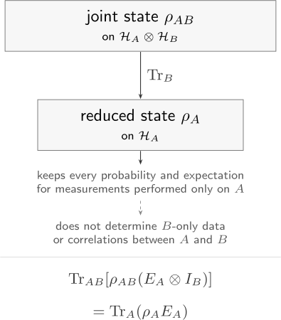
Reduction preserves every statistic of $A$-local effects $E_A\otimes I_B$. It does not retain enough information to reconstruct $B$ or the correlations between the two subsystems.

Product states and correlations

For a product state,

$$\rho_{AB} = \rho_A\otimes\rho_B,$$

one obtains

$$\operatorname{Tr}_B\rho_{AB} = \rho_A\operatorname{Tr}\rho_B = \rho_A.$$

The same local density matrix can arise from very different joint states. Consider

$$\begin{aligned} \rho_{\mathrm{unc}} &= \frac{I_{AB}}{4}, \\ \rho_{\mathrm{cc}} &= \frac12 \left( \lvert00\rangle\langle00\rvert + \lvert11\rangle\langle11\rvert \right), \\ \rho_{\mathrm{ent}} &= \lvert\Phi^+\rangle\langle\Phi^+\rvert. \end{aligned}$$

Here

$$\lvert\Phi^+\rangle = \frac{ \lvert00\rangle+\lvert11\rangle }{\sqrt2}.$$

All three have

$$\rho_A=\rho_B=\frac I2.$$

Yet they have different global structure:

• $\rho_{\mathrm{unc}}$ is uncorrelated;
• $\rho_{\mathrm{cc}}$ is separable but classically correlated;
• $\rho_{\mathrm{ent}}$ is a pure entangled state.

For example,

$$\begin{aligned} \langle Z\otimes Z\rangle_{\mathrm{unc}} &=0, & \langle X\otimes X\rangle_{\mathrm{unc}} &=0, \\ \langle Z\otimes Z\rangle_{\mathrm{cc}} &=1, & \langle X\otimes X\rangle_{\mathrm{cc}} &=0, \\ \langle Z\otimes Z\rangle_{\mathrm{ent}} &=1, & \langle X\otimes X\rangle_{\mathrm{ent}} &=1. \end{aligned}$$

The first correlation separates the product state from the two correlated states; the second separates the classical correlation from the Bell state. Identical marginals do not imply identical joint physics.

Pure joint states and shared spectra

Write a normalized pure state in product bases as

$$\begin{aligned} \lvert\Psi\rangle &= \sum_{i,\mu} C_{i\mu} \lvert i\rangle_A \lvert\mu\rangle_B, \\ 1 &= \sum_{i,\mu} \lvert C_{i\mu}\rvert^2. \end{aligned}$$

The reduced-state matrix elements are

$$\begin{aligned} (\rho_A)_{ij} &= \sum_\mu C_{i\mu}C_{j\mu}^*, \\ (\rho_B)_{\mu\nu} &= \sum_i C_{i\mu}C_{i\nu}^*. \end{aligned}$$

If $C$ denotes the coefficient array with row index $i$ and column index $\mu$, then

$$\rho_A=CC^\dagger, \qquad \rho_B=C^{\mathsf T}C^*.$$

The transpose in the second expression follows from this explicit coefficient convention. Equivalently, $\rho_B$ is the transpose of $C^\dagger C$. Both reduced states have the squared singular values of $C$ as their nonzero eigenvalues.

This is the matrix form of the Schmidt decomposition overview. For a pure bipartite state:

• $\rho_A$ and $\rho_B$ have the same nonzero spectrum;
• their ranks equal the Schmidt rank;
• $\operatorname{Tr}(\rho_A^2)=\operatorname{Tr}(\rho_B^2)$;
• one reduced state is pure exactly when the joint state is a product state;
• a mixed reduced state is equivalent to entanglement across the $A\mid B$ bipartition.

The final statement requires the joint state to be pure. If $\rho_{AB}$ is mixed, a mixed marginal by itself does not certify entanglement.

Partially entangled pair

Consider

$$\begin{aligned} \lvert\Psi\rangle &= \sqrt p\,\lvert00\rangle + e^{i\phi} \sqrt{1-p}\,\lvert11\rangle, \\ 0&\leq p\leq1. \end{aligned}$$

The reductions are

$$\rho_A = \rho_B = p\lvert0\rangle\langle0\rvert + (1-p)\lvert1\rangle\langle1\rvert.$$

The phase $\phi$ is present in the joint coherence but absent from either local state. Their purity is

$$\operatorname{Tr}(\rho_A^2) = p^2+(1-p)^2.$$

The state is a product at $p=0$ or $p=1$, entangled for $0<p<1$, and maximally entangled at $p=1/2$.

Two-qubit matrix example

In the ordered basis

$$\left( \lvert00\rangle, \lvert01\rangle, \lvert10\rangle, \lvert11\rangle \right),$$

consider the physical state

$$\rho_{AB} = \begin{pmatrix} a&0&0&w\\ 0&b&z&0\\ 0&z^*&c&0\\ w^*&0&0&d \end{pmatrix},$$

where

$$\begin{aligned} a,b,c,d&\geq0, & a+b+c+d&=1, \\ \lvert w\rvert^2&\leq ad, & \lvert z\rvert^2&\leq bc. \end{aligned}$$

The reductions are

$$\begin{aligned} \rho_A &= \begin{pmatrix} a+b&0\\ 0&c+d \end{pmatrix}, \\[6pt] \rho_B &= \begin{pmatrix} a+c&0\\ 0&b+d \end{pmatrix}. \end{aligned}$$

The off-diagonal joint entries $w$ and $z$ connect basis states with different labels on the subsystem being traced out, so they vanish from both marginals. They may still affect joint observables and cannot be declared physically irrelevant.

Marginal is not conditional

The reduced state is an unconditioned marginal. It describes local predictions when no outcome on $B$ is selected.

Suppose a measurement on $B$ has Kraus operators $L_b$. The unnormalized conditional state of $A$ for outcome $b$ is

$$\widetilde\rho_{A\mid b} = \operatorname{Tr}_B \left[ (I_A\otimes L_b) \rho_{AB} (I_A\otimes L_b^\dagger) \right].$$

Its probability and normalized state are

$$p(b) = \operatorname{Tr}_A \widetilde\rho_{A\mid b}, \qquad \rho_{A\mid b} = \frac{ \widetilde\rho_{A\mid b} }{ p(b) }$$

when $p(b)>0$. Conditioning depends on the outcome and, for a general measurement, on the measurement instrument.

If the outcome is ignored and

$$\sum_b L_b^\dagger L_b=I_B,$$

then

$$\sum_b \widetilde\rho_{A\mid b} = \rho_A.$$

Thus a local trace-preserving operation on $B$ cannot change the unconditioned state of $A$. The detailed state-update and no-signaling interpretations live in Conditional States and Subsystems and Local Observables.

What reduction preserves and discards

Reduction preserves:

• normalization, Hermiticity, and positivity;
• every probability distribution for a measurement on $A$ alone;
• every expectation value of $M_A\otimes I_B$;
• the nonzero Schmidt spectrum when the joint state is pure.

Reduction does not preserve enough information to recover:

• the state of $B$;
• correlations between $A$ and $B$;
• whether a mixed marginal arose from classical correlation, entanglement, or an uncorrelated mixed preparation;
• relative phases that appear only in joint coherences;
• the original joint state.

The map $\rho_{AB}\mapsto\rho_A$ is many-to-one and has no inverse on the set of joint states. A purification constructs a larger pure state with a chosen marginal, but that construction is highly nonunique.

When $B$ is an uncontrolled environment, $\rho_A(t)$ is the state used to predict accessible observations. Even if $\rho_{AB}(t)$ evolves unitarily, the reduced evolution of $A$ need not be unitary because information and correlations can flow into $B$.

Infinite-dimensional qualification

The formulas above are automatic for finite-dimensional spaces. In infinite dimensions, a density operator is trace class. If $\rho_{AB}$ is trace class, there is a unique trace-class $\rho_A=\operatorname{Tr}_B\rho_{AB}$ satisfying

$$\operatorname{Tr}_A(\rho_A M_A) = \operatorname{Tr}_{AB} \left[ \rho_{AB}(M_A\otimes I_B) \right]$$

for every bounded $M_A$. The basis sum defining the partial trace converges in trace norm. These hypotheses matter: one should not treat arbitrary infinite matrices as though finite-dimensional trace manipulations automatically apply. See Trace-Class and Hilbert–Schmidt Operators for the operator-class background.

Practical workflow

To find and use a reduced density matrix:

1. State the tensor-factor ordering and the subsystem to keep.
2. Form $\rho_{AB}$ if the input is a state vector.
3. Trace over matching row and column labels of the discarded subsystem.
4. Check the output dimension, Hermiticity, positivity, and trace one.
5. Test a simple local expectation value against the joint-state formula.
6. Use $\rho_A$ for local predictions, but return to $\rho_{AB}$ for correlations.
7. Distinguish an unconditioned partial trace from conditioning on a recorded measurement outcome.

Ignorance, Entanglement, and the Meaning of Mixed

A mixed density operator can have more than one physical origin. It may describe classical uncertainty about a preparation. It may describe a subsystem of an entangled pure state. It may describe a subsystem correlated with an environment in both classical and quantum ways.

The density operator alone tells us the statistics of local measurements. It does not always tell us which story produced those statistics.

There is one important special case: if the global state on $AB$ is known to be pure, then a mixed reduced state of $A$ is not merely ignorance about a pure local state of $A$. It is evidence that $A$ is entangled with $B$.

Conversely, Purification shows that every finite-dimensional mixed state can be represented as the reduced state of some larger pure state.

For the open-system distinction between a classical ignorance mixture and a reduced state produced by tracing out correlations, see Proper and Improper Mixtures.

Operational Definition and Uniqueness

For every observable or measurement effect $M_A$ on subsystem $A$, the reduced state must satisfy

$$\operatorname{Tr}_A(\rho_A M_A) = \operatorname{Tr}_{AB} \left[ \rho_{AB} \bigl( M_A\otimes I_B \bigr) \right].$$

This identity can be taken as the operational definition of $\rho_A$. It says that calculating with the smaller state on $\mathcal H_A$ gives exactly the same answer as calculating with the full state and embedding the local operator into $\mathcal H_{AB}$.

The state is unique. In a basis $\{\lvert i\rangle_A\}$, choose the matrix-unit operators

$$M_A^{(ik)} = \lvert k\rangle\langle i\rvert.$$

Then

$$\operatorname{Tr}_A \left( \rho_A M_A^{(ik)} \right) = \langle i\rvert\rho_A\lvert k\rangle.$$

Requiring the local-expectation identity for every pair $(i,k)$ therefore fixes every matrix element of $\rho_A$.

The same identity shows why reduction produces a valid density operator. Setting $M_A=I_A$ gives

$$\operatorname{Tr}_A\rho_A = \operatorname{Tr}_{AB}\rho_{AB} =1.$$

For any $\lvert a\rangle_A$,

$$\begin{aligned} \langle a\rvert\rho_A\lvert a\rangle &= \operatorname{Tr}_{AB} \left[ \rho_{AB} \bigl( \lvert a\rangle\langle a\rvert \otimes I_B \bigr) \right]\\ &\ge0. \end{aligned}$$

Thus $\rho_A$ is positive and, consequently, Hermitian.

Examples

Bell pair

Consider the Bell state

$$\lvert\Phi^+\rangle = \frac{ \lvert00\rangle+\lvert11\rangle }{\sqrt2}.$$

The full density operator is

$$\begin{aligned} \rho_{AB} &= \frac12 \Bigl( \lvert00\rangle\langle00\rvert +\lvert00\rangle\langle11\rvert\\ &\qquad+ \lvert11\rangle\langle00\rvert +\lvert11\rangle\langle11\rvert \Bigr). \end{aligned}$$

Trace out subsystem $B$. The diagonal $B$ overlaps survive, while the cross terms have zero $B$ overlap:

$$\begin{aligned} \rho_A &= \operatorname{Tr}_B\rho_{AB} \\ &= \frac{1}{2} \left( \lvert0\rangle\langle0\rvert +\lvert1\rangle\langle1\rvert \right) \\ &= \frac{I_A}{2}. \end{aligned}$$

Thus a maximally entangled two-qubit pure state has a maximally mixed one-qubit reduced state. An observer measuring only qubit $A$ sees probabilities

$$p(0)=p(1)=\frac{1}{2}$$

in the computational basis, and no local measurement on $A$ can reveal the relative phase in the Bell pair by itself.

The correlations are not gone. They are simply not contained in $\rho_A$ alone. They live in the joint state $\rho_{AB}$.

A continuous family

Consider

$$\begin{aligned} \lvert\Psi(p,\varphi)\rangle &= \sqrt p\,\lvert00\rangle\\ &\quad+ e^{i\varphi}\sqrt{1-p}\,\lvert11\rangle,\\ p&\in[0,1]. \end{aligned}$$

The reduced states are

$$\rho_A=\rho_B = p\lvert0\rangle\langle0\rvert + (1-p)\lvert1\rangle\langle1\rvert.$$

Their purity is

$$\operatorname{Tr}\rho_A^2 = p^2+(1-p)^2.$$

The phase $\varphi$ is absent from either reduced state. It remains observable in joint correlations; for example,

$$\langle \sigma_x\otimes\sigma_x \rangle = 2\sqrt{p(1-p)}\cos\varphi.$$

At $p=0$ or $p=1$, the state is product and the local state is pure. For $0<p<1$, the joint state is entangled and the local state is mixed. At $p=1/2$, both marginals are maximally mixed.

Same marginal, different joint states

Each of the following two-qubit states has $\rho_A=I_A/2$:

$$\rho_{\mathrm{ent}} = \lvert\Phi^+\rangle\langle\Phi^+\rvert,$$ $$\rho_{\mathrm{cc}} = \frac12 \lvert00\rangle\langle00\rvert + \frac12 \lvert11\rangle\langle11\rvert,$$

and

$$\rho_{\mathrm P} = \frac{I_A}{2} \otimes \lvert0\rangle_B{}_B\langle0\rvert.$$

The first is entangled, the second is separable but correlated, and the third is a product state. No measurement on $A$ alone can distinguish them. Joint measurements can.

Reduced-State Dynamics

If only $A$ undergoes a unitary $U_A$, then

$$\rho_A \longmapsto U_A\rho_A U_A^\dagger.$$

If only $B$ undergoes a trace-preserving operation and its outcome is not selected, $\rho_A$ does not change, as shown above.

A joint unitary generally can change the reduced state:

$$\rho_A(t) = \operatorname{Tr}_B \left[ U_{AB}(t)\, \rho_{AB}(0)\, U_{AB}^\dagger(t) \right].$$

Interactions can transfer purity and build correlations, so the reduced evolution need not be unitary. If initial system-environment correlations are present, $\rho_A(0)$ alone may not determine $\rho_A(t)$; the initial joint state can matter.

This is the first bridge from closed-system dynamics to open quantum systems. The present page establishes the kinematics; channels, master equations, and approximations belong to their dedicated volume.

Common mistakes

• Tracing over the subsystem one intended to keep.
• Summing unmatched row and column indices.
• Treating $\rho_A$ as a state vector rather than a density operator.
• Interpreting the partial trace as a projective measurement on $B$.
• Assuming a mixed marginal proves entanglement when the joint state is mixed.
• Assuming equal reduced states imply equal joint states.
• Trying to compute $A$–$B$ correlations from $\rho_A$ alone.
• Forgetting the transpose implied by a chosen coefficient-matrix convention.
• Using finite-dimensional trace formulas for non-trace-class operators.

References

• J. von Neumann, Mathematical Foundations of Quantum Mechanics, Princeton University Press (1955), Ch. IV.
• U. Fano, “Description of States in Quantum Mechanics by Density Matrix and Operator Techniques”, Reviews of Modern Physics 29, 74–93 (1957).
• M. A. Nielsen and I. L. Chuang, Quantum Computation and Quantum Information, 10th anniversary ed., Cambridge University Press (2010), Secs. 2.4 and 2.5.
• J. Watrous, The Theory of Quantum Information, Cambridge University Press (2018), Chs. 1–2.
• J. Preskill, Lecture Notes for Physics 229: Quantum Information and Computation, Chapter 2, Secs. 2.3–2.5.
• H.-P. Breuer and F. Petruccione, The Theory of Open Quantum Systems, Oxford University Press (2002), Secs. 2.1–2.3.
• R. Shankar, Principles of Quantum Mechanics, 2nd ed., Springer (1994).
• A. Peres, Quantum Theory: Concepts and Methods, Kluwer (1995).
• L. E. Ballentine, Quantum Mechanics: A Modern Development, 2nd ed., World Scientific (2014).

Exercises

1. Prove that

$$\operatorname{Tr}_B(\rho_A\otimes\rho_B) = \rho_A$$

for normalized density operators.

Solution

The product rule gives

$$\operatorname{Tr}_B(\rho_A\otimes\rho_B) = \rho_A\operatorname{Tr}\rho_B.$$

Because $\rho_B$ is normalized,

$$\operatorname{Tr}\rho_B=1,$$

and the result follows.

2. Starting from the basis definition of the partial trace, derive

$$\left( \operatorname{Tr}_B X \right)_{ij} = \sum_\mu X_{i\mu,j\mu}.$$

Solution

Insert the basis definition between $\langle i\rvert$ and $\lvert j\rangle$:

$$\begin{aligned} &\langle i\rvert \operatorname{Tr}_B(X) \lvert j\rangle \\ &= \sum_\mu \langle i\rvert \left( I_A\otimes\langle\mu\rvert \right) X \left( I_A\otimes\lvert\mu\rangle \right) \lvert j\rangle \\ &= \sum_\mu \langle i,\mu\rvert X \lvert j,\mu\rangle \\ &= \sum_\mu X_{i\mu,j\mu}. \end{aligned}$$

3. Show directly that $\rho_A=\operatorname{Tr}_B\rho_{AB}$ is positive whenever $\rho_{AB}$ is positive.

Solution

For any $\lvert\alpha\rangle\in\mathcal H_A$ and any orthonormal basis $\{\lvert\mu\rangle\}$ of $B$,

$$\begin{aligned} \langle\alpha\rvert \rho_A \lvert\alpha\rangle &= \sum_\mu \langle\alpha,\mu\rvert \rho_{AB} \lvert\alpha,\mu\rangle. \end{aligned}$$

Every term is nonnegative because $\rho_{AB}\geq0$. Hence the sum is nonnegative for every $\lvert\alpha\rangle$, so $\rho_A\geq0$.

4. Suppose Hermitian trace-one operators $\rho_A$ and $\tau_A$ give the same expectation value for every Hermitian $M_A$. Prove that $\rho_A=\tau_A$.

Solution

Let

$$D=\rho_A-\tau_A.$$

The assumption gives

$$\operatorname{Tr}(DM_A)=0$$

for every Hermitian $M_A$. Since $D$ is Hermitian, choose $M_A=D$:

$$\operatorname{Tr}(D^2)=0.$$

If $d_k$ are the eigenvalues of $D$, then

$$\operatorname{Tr}(D^2) = \sum_k d_k^2.$$

The sum can vanish only when every $d_k=0$. Thus $D=0$ and $\rho_A=\tau_A$.

5. For

$$\lvert\Psi\rangle = \sqrt p\,\lvert00\rangle + e^{i\phi} \sqrt{1-p}\,\lvert11\rangle,$$

compute both reduced states, their purity, and the values of $p$ for which the joint state is entangled.

Solution

The joint density operator contains diagonal terms

$$p\lvert00\rangle\langle00\rvert + (1-p)\lvert11\rangle\langle11\rvert$$

and two cross terms with different $B$ labels. The cross terms vanish under $\operatorname{Tr}_B$, giving

$$\rho_A = p\lvert0\rangle\langle0\rvert + (1-p)\lvert1\rangle\langle1\rvert.$$

By symmetry, $\rho_B=\rho_A$. Their purity is

$$\operatorname{Tr}(\rho_A^2) = p^2+(1-p)^2.$$

The reduction is pure only for $p=0$ or $p=1$. Because the joint state is pure, it is entangled exactly when the reduction is mixed:

$$0<p<1.$$

6. Verify that $\rho_{\mathrm{unc}}$, $\rho_{\mathrm{cc}}$, and $\rho_{\mathrm{ent}}$ from the text all have marginal $I/2$ on $A$. Then explain how $Z\otimes Z$ and $X\otimes X$ distinguish them.

Solution

For $I_{AB}/4$,

$$\operatorname{Tr}_B \left( \frac{I_A\otimes I_B}{4} \right) = \frac{I_A}{2}.$$

For $\rho_{\mathrm{cc}}$, tracing either $\lvert00\rangle\langle00\rvert$ or $\lvert11\rangle\langle11\rvert$ over $B$ leaves the corresponding $A$ projector, so the equal mixture gives $I_A/2$. The Bell-state cross terms vanish under the partial trace, giving the same result.

Their correlations are

$$\begin{aligned} \langle Z\otimes Z\rangle &= 0,\ 1,\ 1, \\ \langle X\otimes X\rangle &= 0,\ 0,\ 1, \end{aligned}$$

in the order product, classically correlated, entangled. Thus local marginals agree while joint observables distinguish the states.

7. Reduce the two-qubit matrix

$$\rho_{AB} = \begin{pmatrix} a&0&0&w\\ 0&b&z&0\\ 0&z^*&c&0\\ w^*&0&0&d \end{pmatrix}$$

over $B$ and over $A$.

Solution

For $\rho_A$, sum entries with matching $B$ labels:

$$\begin{aligned} (\rho_A)_{00} &= \rho_{00,00}+\rho_{01,01} = a+b, \\ (\rho_A)_{11} &= \rho_{10,10}+\rho_{11,11} = c+d. \end{aligned}$$

The off-diagonal entries vanish, so

$$\rho_A = \begin{pmatrix} a+b&0\\ 0&c+d \end{pmatrix}.$$

Similarly,

$$\rho_B = \begin{pmatrix} a+c&0\\ 0&b+d \end{pmatrix}.$$

The entries $w$ and $z$ connect unequal labels on either traced subsystem and do not appear in the marginals.

8. The Bell state $\lvert\Phi^+\rangle$ is measured in the $Z$ basis on subsystem $B$. Find the conditional states of $A$ for both outcomes and their unconditioned average.

Solution

Outcome $0$ occurs with probability $1/2$ and leaves

$$\rho_{A\mid0} = \lvert0\rangle\langle0\rvert.$$

Outcome $1$ also occurs with probability $1/2$ and leaves

$$\rho_{A\mid1} = \lvert1\rangle\langle1\rvert.$$

If the outcome is not retained, the average state is

$$\begin{aligned} \rho_A &= \frac12\rho_{A\mid0} + \frac12\rho_{A\mid1} \\ &= \frac12 \left( \lvert0\rangle\langle0\rvert + \lvert1\rangle\langle1\rvert \right) \\ &= \frac I2. \end{aligned}$$

Conditioning changes the state assigned using a known outcome; ignoring the outcome returns the original reduced state.

Additional exercises retained from the earlier canonical treatment

1. Let $\rho_{AB}=\rho_A\otimes\rho_B$. Show that tracing over $B$ returns $\rho_A$.

Solution

Using trace factorization,

$$\operatorname{Tr}_B(\rho_A\otimes\rho_B) = \rho_A\,\operatorname{Tr}_B\rho_B.$$

Since $\rho_B$ is normalized, $\operatorname{Tr}_B\rho_B=1$, so the result is $\rho_A$.

2. Compute the reduced state of $A$ for

$$\rho_{AB} = \frac12 \lvert00\rangle\langle00\rvert + \frac12 \lvert11\rangle\langle11\rvert.$$

Solution

Trace over the second qubit:

$$\rho_A = \frac12 \lvert0\rangle\langle0\rvert + \frac12 \lvert1\rangle\langle1\rvert = \frac12 I.$$

The state is locally maximally mixed, even though the global state is not the Bell state.

3. Suppose a two-qubit pure state has reduced density operator $\rho_A=I/2$. Is the pure joint state product?

Solution

No. If a pure bipartite state were product, each subsystem would be pure. But $I/2$ is mixed because

$$\operatorname{Tr}(\rho_A^2) = \operatorname{Tr}\left(\frac14 I\right) = \frac12 < 1.$$

Therefore the pure joint state is entangled across the two-qubit split.

Additional subsystem-state exercises

1. Let $\rho_{AB}=\rho_A\otimes\rho_B$ with $\operatorname{Tr}\rho_B=1$. Compute $\operatorname{Tr}_B\rho_{AB}$.

Solution

Using trace factorization,

$$\operatorname{Tr}_B(\rho_A\otimes\rho_B) = \rho_A\,\operatorname{Tr}(\rho_B) = \rho_A.$$

2. Compute the reduced state of qubit $A$ for

$$\lvert\Psi\rangle = \alpha\lvert00\rangle+\beta\lvert11\rangle, \qquad \lvert\alpha\rvert^2+\lvert\beta\rvert^2=1.$$

Solution

The density operator contains four terms:

$$\begin{aligned} \rho_{AB} &= \lvert\alpha\rvert^2 \lvert00\rangle\langle00\rvert + \alpha\beta^* \lvert00\rangle\langle11\rvert \\ &\quad + \alpha^*\beta \lvert11\rangle\langle00\rvert + \lvert\beta\rvert^2 \lvert11\rangle\langle11\rvert. \end{aligned}$$

Tracing out $B$ removes the cross terms because $\langle0\vert1\rangle=0$, giving

$$\rho_A = \lvert\alpha\rvert^2 \lvert0\rangle\langle0\rvert + \lvert\beta\rvert^2 \lvert1\rangle\langle1\rvert.$$

3. Show that the reduced state of either qubit in $\lvert\Phi^+\rangle$ is $I/2$.

Solution

The page computed $\rho_A=I_A/2$. By symmetry under exchanging the two qubits, the same calculation gives

$$\rho_B=\frac{I_B}{2}.$$

4. Let $M_A$ be an observable on subsystem $A$. What is the composite-system observable corresponding to measuring $M_A$ while doing nothing to $B$?

Solution

The corresponding observable on $\mathcal H_A\otimes\mathcal H_B$ is

$$M_A\otimes I_B.$$

The reduced state $\rho_A$ is defined so that the expectation value of this observable agrees with $\operatorname{Tr}_A(\rho_A M_A)$.

5. A qubit–qutrit pure state is

$$\lvert\Omega\rangle = \frac{ \lvert0,0\rangle +\lvert1,1\rangle +\lvert1,2\rangle }{\sqrt3}.$$

Find its coefficient matrix, $\rho_A$, and $\rho_B$. Verify that the two reduced states have the same nonzero eigenvalues.

Solution

With $A$ indexing rows and $B$ indexing columns,

$$C = \frac{1}{\sqrt3} \begin{pmatrix} 1&0&0\\ 0&1&1 \end{pmatrix}.$$

Therefore

$$\rho_A = CC^\dagger = \frac13 \begin{pmatrix} 1&0\\ 0&2 \end{pmatrix},$$

and

$$\rho_B = C^{\mathsf T}C^* = \frac13 \begin{pmatrix} 1&0&0\\ 0&1&1\\ 0&1&1 \end{pmatrix}.$$

The eigenvalues of $\rho_A$ are $1/3$ and $2/3$. The qutrit state has the same two nonzero eigenvalues plus one zero eigenvalue:

$$\operatorname{spec}(\rho_B) = \left\{ \frac23,\frac13,0 \right\}.$$

6. Let $U_B$ be a unitary on $B$ and

$$\rho'_{AB} = \bigl( I_A\otimes U_B \bigr) \rho_{AB} \bigl( I_A\otimes U_B^\dagger \bigr).$$

Show that $\operatorname{Tr}_B\rho'_{AB}=\rho_A$.

Solution

Use cyclicity of the partial trace with respect to operators acting only on the traced subsystem:

$$\begin{aligned} \operatorname{Tr}_B\rho'_{AB} &= \operatorname{Tr}_B \left[ \rho_{AB} \bigl( I_A\otimes U_B^\dagger U_B \bigr) \right]\\ &= \operatorname{Tr}_B \left[ \rho_{AB} \bigl( I_A\otimes I_B \bigr) \right]\\ &= \rho_A. \end{aligned}$$

A remote unitary can change correlations and conditional states, but not the unconditioned marginal of $A$.

7. For

$$\lvert\Phi_\varphi\rangle = \frac{ \lvert00\rangle + e^{i\varphi}\lvert11\rangle }{\sqrt2},$$

show that $\rho_A=\rho_B=I/2$ for every $\varphi$, while

$$\langle \sigma_x\otimes\sigma_x \rangle = \cos\varphi.$$

Solution

The joint density operator contains diagonal terms and phase-dependent cross terms. The cross terms vanish under either partial trace because $\langle0\vert1\rangle=0$. Hence

$$\rho_A=\rho_B=\frac12 I$$

independently of $\varphi$.

Since

$$\begin{aligned} \sigma_x\otimes\sigma_x \lvert00\rangle &= \lvert11\rangle,\\ \sigma_x\otimes\sigma_x \lvert11\rangle &= \lvert00\rangle. \end{aligned}$$

the joint expectation is

$$\begin{aligned} \langle \sigma_x\otimes\sigma_x \rangle &= \frac12 \left( e^{i\varphi}+e^{-i\varphi} \right)\\ &= \cos\varphi. \end{aligned}$$

The phase is locally invisible but jointly observable.

8. Assess the claim: “If $\rho_A$ is mixed, then $A$ is entangled with $B$.”

Solution

The claim is true only when the joint state $\rho_{AB}$ is known to be pure. For a pure bipartite state, a mixed marginal is equivalent to Schmidt rank greater than one and therefore to entanglement.

For a mixed joint state, the claim is false. For example,

$$\rho_{AB} = \frac{I_A}{2} \otimes \lvert0\rangle_B{}_B\langle0\rvert$$

is a product state, yet

$$\rho_A=\frac{I_A}{2}$$

is mixed. Local mixedness alone does not identify its global origin.