Purification

This is the canonical treatment of purification, including constructions, nonuniqueness, ensemble meaning, dilation links, and infinite-dimensional qualifications. For a density-operator-motivated first encounter, use Purification Overview.

Purification expresses every density operator as the reduced state of a pure state on a larger Hilbert space. If system $A$ has state $\rho_A$, one may introduce a reference system $R$ and find a normalized vector $\lvert\Psi\rangle_{AR}$ such that

$$\rho_A = \operatorname{Tr}_R \bigl( \lvert\Psi\rangle\langle\Psi\rvert_{AR} \bigr).$$

This representation connects mixed states, entanglement, ensemble decompositions, and open-system models. It is a mathematical existence statement, not evidence that $\rho_A$ has one privileged hidden environment or one uniquely determined preparation history.

Definition and Scope

Let $\rho_A$ be a density operator on a finite-dimensional Hilbert space $\mathcal H_A$. A purification of $\rho_A$ consists of

1. an auxiliary Hilbert space $\mathcal H_R$, and
2. a normalized vector $\lvert\Psi\rangle_{AR}\in\mathcal H_A\otimes\mathcal H_R$

for which

$$\operatorname{Tr}_R \bigl( \lvert\Psi\rangle\langle\Psi\rvert_{AR} \bigr) = \rho_A.$$

The condition says more than merely matching eigenvalues. It guarantees that every observable $M_A$ acting locally on $A$ has the same expectation value in the two descriptions:

$$\begin{aligned} \operatorname{Tr}_A(\rho_A M_A) &= \operatorname{Tr}_{AR} \bigl( \lvert\Psi\rangle\langle\Psi\rvert_{AR} \\ &\qquad{}\times (M_A\otimes I_R) \bigr) \\ &= \langle\Psi\rvert (M_A\otimes I_R) \lvert\Psi\rangle. \end{aligned}$$

No experiment confined to $A$ can distinguish $\rho_A$ from its description as part of the larger pure state. Access to $R$, or to correlations between $A$ and $R$, supplies additional information.

The label $R$ is deliberately neutral. Depending on the problem it may denote a mathematical reference, a controllable ancilla, an inaccessible environment, or a genuine second subsystem. Purification alone does not choose among these interpretations.

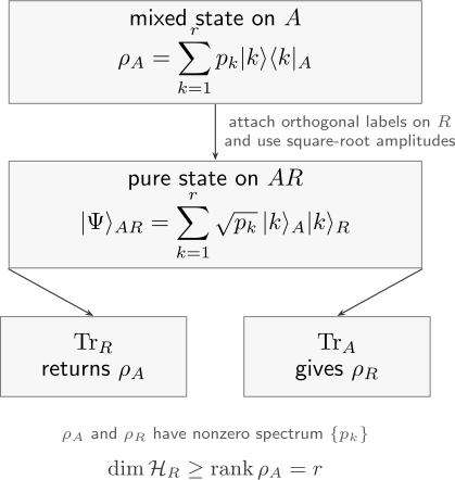
The spectral construction assigns one orthogonal reference label to each nonzero eigenvalue. The smallest purifying space has dimension $\operatorname{rank}\rho_A$.

Finite-Dimensional Existence Theorem

Purification theorem. Every finite-dimensional density operator has a purification. If

$$r=\operatorname{rank}\rho_A,$$

then a reference space of dimension $r$ is sufficient and no smaller reference space can purify $\rho_A$.

To prove existence, use the spectral decomposition on the support of $\rho_A$:

$$\begin{aligned} \rho_A &= \sum_{k=1}^{r} p_k \lvert k\rangle_A\langle k\rvert_A, \\ p_k&>0, \qquad \sum_{k=1}^{r}p_k=1. \end{aligned}$$

Choose orthonormal vectors $\{\lvert k\rangle_R\}_{k=1}^r$ and define

$$\lvert\Psi_\rho\rangle_{AR} = \sum_{k=1}^{r} \sqrt{p_k}\, \lvert k\rangle_A\lvert k\rangle_R.$$

Normalization follows immediately:

$$\begin{aligned} \langle\Psi_\rho\vert\Psi_\rho\rangle &= \sum_{j,k=1}^{r} \sqrt{p_jp_k}\, \langle j\vert k\rangle_A \\ &\qquad{}\times \langle j\vert k\rangle_R \\ &= \sum_{k=1}^{r}p_k =1. \end{aligned}$$

For the reduced state, expand the projector and trace the reference factor:

$$\begin{aligned} \operatorname{Tr}_R \bigl( \lvert\Psi_\rho\rangle \langle\Psi_\rho\rvert \bigr) &= \sum_{j,k=1}^{r} \sqrt{p_jp_k}\, \lvert j\rangle_A\langle k\rvert_A \\ &\quad{}\times \operatorname{Tr} \bigl( \lvert j\rangle_R\langle k\rvert_R \bigr) \\ &= \sum_{j,k=1}^{r} \sqrt{p_jp_k}\, \delta_{jk} \lvert j\rangle_A\langle k\rvert_A \\ &= \sum_{k=1}^{r} p_k \lvert k\rangle_A\langle k\rvert_A = \rho_A. \end{aligned}$$

This proves existence. It also displays the nonzero eigenvalues of the other marginal:

$$\rho_R = \operatorname{Tr}_A \bigl( \lvert\Psi_\rho\rangle \langle\Psi_\rho\rvert \bigr) = \sum_{k=1}^{r} p_k \lvert k\rangle_R\langle k\rvert_R.$$

The rank bound follows from the Schmidt decomposition. Any pure state on $A R$ has at most $\dim\mathcal H_R$ nonzero Schmidt coefficients, while the rank of its reduced state on $A$ equals its Schmidt rank. Therefore

$$\dim\mathcal H_R \ge \operatorname{rank}\rho_A.$$

The spectral construction saturates this inequality.

Square-Root Construction

There is a basis-dependent formula that avoids diagonalizing $\rho_A$. Let $\mathcal H_R$ be a copy of the $d$-dimensional space $\mathcal H_A$, choose corresponding orthonormal bases, and introduce the unnormalized maximally correlated vector

$$\lvert\Omega\rangle_{AR} = \sum_{j=1}^{d} \lvert j\rangle_A\lvert j\rangle_R.$$

Then

$$\lvert\Psi_\rho\rangle_{AR} = \bigl( \sqrt{\rho_A}\otimes I_R \bigr) \lvert\Omega\rangle_{AR}$$

is a purification. Its norm is

$$\begin{aligned} \langle\Psi_\rho\vert\Psi_\rho\rangle &= \langle\Omega\rvert (\rho_A\otimes I_R) \lvert\Omega\rangle \\ &= \operatorname{Tr}\rho_A =1. \end{aligned}$$

Writing $(\sqrt{\rho_A})_{jk}=\langle j\vert\sqrt{\rho_A}\vert k\rangle$ gives

$$\lvert\Psi_\rho\rangle = \sum_{j,k=1}^{d} (\sqrt{\rho_A})_{jk} \lvert j\rangle_A\lvert k\rangle_R.$$

Tracing $R$ contracts the shared index $k$:

$$\begin{aligned} \operatorname{Tr}_R \bigl( \lvert\Psi_\rho\rangle \langle\Psi_\rho\rvert \bigr) &= \sum_{j,j',k} (\sqrt{\rho_A})_{jk} (\sqrt{\rho_A})_{j'k}^{*} \\ &\quad{}\times \lvert j\rangle\langle j'\rvert_A \\ &= \sqrt{\rho_A}\, \sqrt{\rho_A}^{\dagger} = \rho_A. \end{aligned}$$

Because $\sqrt{\rho_A}$ is positive and therefore Hermitian, the last product is exactly $\rho_A$. This construction is useful in matrix calculations and anticipates state–operator correspondences, but it depends on the chosen identification of bases in $A$ and $R$.

Ensemble-Labeled Purifications

Purification does not require an eigenstate ensemble. Suppose

$$\begin{aligned} \rho_A &= \sum_{j=1}^{m} q_j \lvert\psi_j\rangle \langle\psi_j\rvert, \\ q_j&\ge0, \qquad \sum_{j=1}^{m}q_j=1. \end{aligned}$$

where the normalized states $\lvert\psi_j\rangle$ need not be orthogonal. Introduce orthonormal labels $\{\lvert j\rangle_R\}$ and set

$$\lvert\Phi\rangle_{AR} = \sum_{j=1}^{m} \sqrt{q_j}\, \lvert\psi_j\rangle_A \lvert j\rangle_R.$$

Then

$$\begin{aligned} \operatorname{Tr}_R \bigl( \lvert\Phi\rangle \langle\Phi\rvert \bigr) &= \sum_{j,k} \sqrt{q_jq_k}\, \lvert\psi_j\rangle \langle\psi_k\rvert \langle k\vert j\rangle_R \\ &= \sum_j q_j \lvert\psi_j\rangle \langle\psi_j\rvert = \rho_A. \end{aligned}$$

Unlike the spectral construction, this expression is generally not a Schmidt decomposition because the $\lvert\psi_j\rangle$ need not be orthogonal.

The finite-dimensional Hughston–Jozsa–Wootters theorem sharpens this observation: every pure-state ensemble decomposition of $\rho_A$ can be generated by a suitable measurement on a purifying system, with the measurement outcome retained as a classical label. If that outcome is ignored, the state of $A$ remains $\rho_A$. This is why an ensemble records a preparation procedure rather than an additional intrinsic decomposition of the density operator. See Ensembles and Preparation Procedures and Conditional States.

Qubit Geometry

Write a qubit density operator in Bloch form:

$$\begin{aligned} \rho_A &= \frac12 \bigl( I+\boldsymbol r\mathbin{\cdot}\boldsymbol\sigma \bigr), \\ r&=\lVert\boldsymbol r\rVert, \qquad 0\le r\le1. \end{aligned}$$

For $r>0$, let $\lvert\boldsymbol n,+\rangle$ and $\lvert\boldsymbol n,-\rangle$ be eigenstates of $\boldsymbol n\mathbin{\cdot}\boldsymbol\sigma$, where $\boldsymbol n=\boldsymbol r/r$. The eigenvalues are

$$\lambda_\pm = \frac{1\pm r}{2},$$

so a two-qubit purification is

$$\begin{aligned} \lvert\Psi_{\boldsymbol r}\rangle_{AR} &= \sqrt{\frac{1+r}{2}}\, \lvert\boldsymbol n,+\rangle_A \lvert0\rangle_R \\ &\quad+ \sqrt{\frac{1-r}{2}}\, \lvert\boldsymbol n,-\rangle_A \lvert1\rangle_R. \end{aligned}$$

At $r=1$, one eigenvalue vanishes and the purification is a product state after discarding the unused reference direction. At $r=0$, the qubit is maximally mixed and the direction $\boldsymbol n$ is irrelevant; every minimal purification is maximally entangled. One choice is

$$\begin{aligned} \lvert\Phi^+\rangle_{AR} &= \frac{ \lvert00\rangle+\lvert11\rangle }{ \sqrt2 }, \\ \operatorname{Tr}_R \bigl( \lvert\Phi^+\rangle \langle\Phi^+\rvert \bigr) &= \frac I2. \end{aligned}$$

Thus the Bloch radius measures both local purity and, for a purifying two-qubit pure state, the imbalance of the Schmidt coefficients:

$$\operatorname{Tr}(\rho_A^2) = \lambda_+^2+\lambda_-^2 = \frac{1+r^2}{2}.$$

The geometry of $\boldsymbol r$ itself is developed in Bloch Sphere.

What Nonuniqueness Means

If $\lvert\Psi\rangle_{AR}$ purifies $\rho_A$ and $U_R$ is unitary, then

$$\lvert\Psi_U\rangle_{AR} = (I_A\otimes U_R) \lvert\Psi\rangle_{AR}$$

is another purification. Indeed,

$$\begin{aligned} &\operatorname{Tr}_R \left[ (I_A\otimes U_R) \lvert\Psi\rangle\langle\Psi\rvert (I_A\otimes U_R^\dagger) \right] \\ &\qquad= \operatorname{Tr}_R \bigl( \lvert\Psi\rangle\langle\Psi\rvert \bigr) = \rho_A. \end{aligned}$$

Several distinctions matter:

• Changing the reference basis changes the vector in the larger Hilbert space but not the local state on $A$.
• A degenerate spectral decomposition allows different eigenbases, but it does not create inequivalent local density operators.
• Different physical preparation histories can yield the same $\rho_A$ without being identified by purification.
• The density operator fixes all local statistics, not a unique joint state with a real environment.

For example,

$$\begin{aligned} \frac I2 &= \frac12 \bigl( \lvert0\rangle\langle0\rvert + \lvert1\rangle\langle1\rvert \bigr) \\ &= \frac12 \bigl( \lvert+\rangle\langle+\rvert + \lvert-\rangle\langle-\rvert \bigr). \end{aligned}$$

Measuring the reference qubit of $\lvert\Phi^+\rangle$ in the computational basis realizes the first conditional ensemble; measuring it in the $X$ basis realizes the second. Discarding the outcome gives $I/2$ in either case.

Entanglement and Mixedness

For a pure state on $A R$, the Schmidt decomposition gives

$$\lvert\Psi\rangle_{AR} = \sum_{k=1}^{r} \sqrt{p_k}\, \lvert a_k\rangle_A \lvert r_k\rangle_R.$$

Its reduced states have the same nonzero eigenvalues:

$$\begin{aligned} \rho_A &= \sum_{k=1}^{r} p_k \lvert a_k\rangle\langle a_k\rvert, \\ \rho_R &= \sum_{k=1}^{r} p_k \lvert r_k\rangle\langle r_k\rvert. \end{aligned}$$

Consequently:

• $\rho_A$ is pure exactly when the Schmidt rank is one.
• $\rho_A$ is mixed exactly when every purification is entangled between $A$ and $R$.
• The two marginals have equal purity, $\operatorname{Tr}(\rho_A^2)=\operatorname{Tr}(\rho_R^2)$.
• Their von Neumann entropies agree whenever those entropies are finite.

For a globally pure bipartite state, the entropy of either marginal therefore quantifies entanglement across the bipartition. The same statement is not valid for a general mixed joint state, where local mixedness can reflect both classical uncertainty and quantum correlations. See Entropy Overview and Subsystem Entropy.

State Purification and Channel Dilation

Purification is a statement about one state. A closely related but distinct theorem represents an entire quantum channel by reversible evolution on a larger space. In finite dimensions, a channel $\mathcal E$ admits an isometry

$$V: \mathcal H_A \longrightarrow \mathcal H_B\otimes\mathcal H_E, \qquad V^\dagger V=I_A,$$

such that

$$\mathcal E(\rho_A) = \operatorname{Tr}_E \bigl( V\rho_A V^\dagger \bigr).$$

Equivalently, one may append an environment in a fixed pure state, apply a unitary on a sufficiently large joint space, and ignore part of the output. This Stinespring representation explains why the same pattern appears repeatedly:

1. enlarge the Hilbert space,
2. use pure-state or reversible structure there,
3. take a partial trace to recover the accessible description.

The distinction is important. A purification reproduces one specified density operator; a channel dilation must reproduce the map for every input state and preserve all correlations with untouched reference systems.

Infinite-Dimensional Qualification

The finite-dimensional proof extends to a positive trace-class operator on a separable Hilbert space. Such a density operator has a countable spectral resolution,

$$\rho_A = \sum_{k} p_k \lvert k\rangle\langle k\rvert, \qquad \sum_k p_k=1,$$

and the same series with coefficients $\sqrt{p_k}$ defines a normalized purification on a suitable reference space. The required reference rank may now be infinite, and convergence is understood in the Hilbert-space and trace-class senses.

There are settings, especially algebraic formulations of quantum field theory, in which a state is defined as a positive normalized functional and need not be represented by a density operator on a preferred tensor factor. The elementary theorem should not be exported to those settings without checking the representation and subsystem assumptions.

Practical Workflow

Given a finite-dimensional $\rho_A$:

1. Check positivity and $\operatorname{Tr}\rho_A=1$.
2. Diagonalize $\rho_A$ if a Schmidt-form purification is wanted.
3. Keep only nonzero eigenvalues to identify the minimal reference dimension.
4. Attach orthonormal reference labels and use square-root amplitudes.
5. Verify normalization.
6. Trace the reference system explicitly.
7. Interpret $R$ only after the mathematical construction is complete.

For numerical work, the square-root construction is often convenient. For conceptual work, the spectral construction makes rank, entanglement, and entropy transparent.

Thermofield and QFT Preview

Thermal states also admit purifications. If

$$\rho_\beta = \frac{e^{-\beta H}}{Z} = \sum_n p_n \lvert n\rangle\langle n\rvert, \qquad p_n = \frac{e^{-\beta E_n}}{Z},$$

then a standard purification on two copies of the Hilbert space is

$$\lvert\mathrm{TFD}(\beta)\rangle = \sum_n \sqrt{p_n}\, \lvert n\rangle_L\lvert n\rangle_R = \frac{1}{\sqrt Z} \sum_n e^{-\beta E_n/2} \lvert n\rangle_L\lvert n\rangle_R.$$

Tracing over the right copy gives the thermal density operator on the left copy:

$$\operatorname{Tr}_R \bigl( \lvert\mathrm{TFD}(\beta)\rangle \langle\mathrm{TFD}(\beta)\rvert \bigr) = \rho_{\beta,L}.$$

This thermofield-double construction is one bridge from ordinary density operators to finite-temperature many-body physics and QFT. The details depend on the Hamiltonian, spectrum, and field-theory setting; this page only gives the purification pattern.

Common Mistakes

• Calling an ensemble decomposition itself a purification. A purification is one vector on a larger tensor-product space.
• Using amplitudes $p_k$ instead of $\sqrt{p_k}$.
• Omitting orthogonality of the reference labels in an ensemble-labeled construction.
• Assuming the purifying system must be a literal environment.
• Treating a purification as unique.
• Choosing $\dim\mathcal H_R<\operatorname{rank}\rho_A$.
• Forgetting that a product purification exists only for a pure $\rho_A$.
• Inferring that a mixed subsystem makes the total state mixed.
• Confusing state purification with a channel dilation.
• Applying the finite-dimensional density-matrix theorem where no subsystem tensor factor or density operator has been specified.

Cross-Links

• Density Operators
• Pure vs Mixed States
• Ensembles and Preparation Procedures
• Trace Rule for Expectation Values
• Bloch Sphere
• Reduced Density Matrices
• Entropy Overview
• Partial Trace
• Schmidt Decomposition
• Conditional States
• Subsystem Entropy
• Spectral Decomposition

References

• M. A. Nielsen and I. L. Chuang, Quantum Computation and Quantum Information, 10th anniversary edition, Cambridge University Press, 2010, Chapters 2 and 8. Cambridge DOI.
• J. Watrous, The Theory of Quantum Information, Cambridge University Press, 2018, Sections 2.1–2.2. Author’s book page and manuscript.
• L. P. Hughston, R. Jozsa, and W. K. Wootters, “A complete classification of quantum ensembles having a given density matrix,” Physics Letters A 183, 14–18 (1993). DOI: 10.1016/0375-9601(93)90880-9.
• W. F. Stinespring, “Positive functions on C*-algebras,” Proceedings of the American Mathematical Society 6, 211–216 (1955). DOI: 10.1090/S0002-9939-1955-0069403-4.
• A. Uhlmann, “The Transition Probability in the State Space of a C*-Algebra,” Reports on Mathematical Physics 9, 273–279 (1976).
• A. Peres, Quantum Theory: Concepts and Methods, Kluwer (1995).
• H. Umezawa, Advanced Field Theory: Micro, Macro, and Thermal Physics, American Institute of Physics (1993).

Exercises

1. Let

$$\rho_A = \sum_{k=1}^{r} p_k \lvert k\rangle\langle k\rvert$$

with $p_k>0$. Verify both normalization and the reduced-state condition for the spectral purification.

Solution

Set

$$\lvert\Psi\rangle_{AR} = \sum_{k=1}^{r} \sqrt{p_k}\, \lvert k\rangle_A\lvert k\rangle_R.$$

Orthonormality in both factors gives

$$\langle\Psi\vert\Psi\rangle = \sum_{j,k} \sqrt{p_jp_k}\, \delta_{jk}\delta_{jk} = \sum_k p_k =1.$$

For the partial trace,

$$\begin{aligned} \operatorname{Tr}_R \bigl( \lvert\Psi\rangle\langle\Psi\rvert \bigr) &= \sum_{j,k} \sqrt{p_jp_k}\, \lvert j\rangle\langle k\rvert_A \\ &\quad{}\times \langle k\vert j\rangle_R \\ &= \sum_k p_k \lvert k\rangle\langle k\rvert_A = \rho_A. \end{aligned}$$

2. Prove that a density operator of rank $r$ cannot be purified using a reference space of dimension smaller than $r$.

Solution

Any vector on $\mathcal H_A\otimes\mathcal H_R$ has Schmidt rank at most

$$\min \bigl( \dim\mathcal H_A, \dim\mathcal H_R \bigr).$$

For a pure bipartite state, the rank of either reduced density operator equals the Schmidt rank. If the reduced state on $A$ has rank $r$, then the purifying vector has Schmidt rank $r$, so

$$\dim\mathcal H_R\ge r.$$

The spectral construction uses exactly $r$ orthogonal reference vectors, so the bound is attainable.

3. Prove the square-root construction directly in a fixed basis.

Solution

With

$$\lvert\Omega\rangle = \sum_k \lvert k\rangle_A\lvert k\rangle_R,$$

the proposed vector has coefficients

$$\lvert\Psi_\rho\rangle = \sum_{j,k} (\sqrt\rho)_{jk} \lvert j\rangle_A\lvert k\rangle_R.$$

Tracing $R$ gives

$$\begin{aligned} \operatorname{Tr}_R \bigl( \lvert\Psi_\rho\rangle \langle\Psi_\rho\rvert \bigr) &= \sum_{j,j',k} (\sqrt\rho)_{jk} (\sqrt\rho)_{j'k}^{*} \\ &\quad{}\times \lvert j\rangle\langle j'\rvert \\ &= \sqrt\rho\,\sqrt\rho^{\dagger} = \rho. \end{aligned}$$

Taking the trace of this equality gives $\langle\Psi_\rho\vert\Psi_\rho\rangle=\operatorname{Tr}\rho=1$.

4. The nonorthogonal ensemble

$$\rho = \frac12 \lvert0\rangle\langle0\rvert + \frac12 \lvert+\rangle\langle+\rvert$$

is given. Construct an ensemble-labeled purification and verify it.

Solution

Choose orthogonal reference states $\lvert0\rangle_R$ and $\lvert1\rangle_R$:

$$\lvert\Phi\rangle_{AR} = \frac{1}{\sqrt2} \left( \lvert0\rangle_A\lvert0\rangle_R + \lvert+\rangle_A\lvert1\rangle_R \right).$$

The vector is normalized because the reference labels are orthogonal:

$$\langle\Phi\vert\Phi\rangle = \frac12+\frac12 =1.$$

When $R$ is traced out, the cross terms contain $\langle0\vert1\rangle_R$ or $\langle1\vert0\rangle_R$ and vanish. The remaining terms are

$$\operatorname{Tr}_R \bigl( \lvert\Phi\rangle\langle\Phi\rvert \bigr) = \frac12 \lvert0\rangle\langle0\rvert + \frac12 \lvert+\rangle\langle+\rvert.$$

The two states on $A$ need not be orthogonal because orthogonality of the labels on $R$ performs the required bookkeeping.

5. Show that a unitary on the reference system cannot change the reduced state on $A$.

Solution

Choose any orthonormal basis $\{\lvert a\rangle_R\}$. For an operator $X_{AR}$,

$$\begin{aligned} \operatorname{Tr}_R X_{AR} &= \sum_a (I_A\otimes\langle a\rvert) X_{AR} \\ &\quad{}\times (I_A\otimes\lvert a\rangle). \end{aligned}$$

Apply this to

$$X_{AR} = (I_A\otimes U_R) \lvert\Psi\rangle\langle\Psi\rvert (I_A\otimes U_R^\dagger).$$

The vectors $U_R^\dagger\lvert a\rangle$ also form an orthonormal basis, so the basis sum is exactly the original partial trace. Therefore

$$\operatorname{Tr}_R X_{AR} = \operatorname{Tr}_R \bigl( \lvert\Psi\rangle\langle\Psi\rvert \bigr) = \rho_A.$$

6. For a qubit with Bloch radius $r$, determine the Schmidt coefficients of a minimal purification, its reduced purity, and the values of $r$ for which the purification is entangled.

Solution

The eigenvalues of the qubit state are

$$\lambda_\pm = \frac{1\pm r}{2}.$$

Hence the Schmidt coefficients are

$$\sqrt{\lambda_+} = \sqrt{\frac{1+r}{2}}, \qquad \sqrt{\lambda_-} = \sqrt{\frac{1-r}{2}}.$$

The reduced purity is

$$\begin{aligned} \operatorname{Tr}(\rho^2) &= \lambda_+^2+\lambda_-^2 \\ &= \frac{(1+r)^2+(1-r)^2}{4} \\ &= \frac{1+r^2}{2}. \end{aligned}$$

Both Schmidt coefficients are nonzero when $0\le r<1$, so every minimal purification is entangled in that range. At $r=1$, one coefficient vanishes and the purification is a product state.

7. Starting from $\lvert\Phi^+\rangle=(\lvert00\rangle+\lvert11\rangle)/\sqrt2$, show how measurements of $R$ produce two different ensembles of $I/2$.

Solution

In the computational basis,

$$\lvert\Phi^+\rangle = \frac{ \lvert0\rangle_A\lvert0\rangle_R + \lvert1\rangle_A\lvert1\rangle_R }{ \sqrt2 }.$$

A measurement of $R$ in that basis prepares $\lvert0\rangle_A$ or $\lvert1\rangle_A$, each with probability $1/2$.

Using

$$\lvert\Phi^+\rangle = \frac{ \lvert+\rangle_A\lvert+\rangle_R + \lvert-\rangle_A\lvert-\rangle_R }{ \sqrt2 },$$

a measurement of $R$ in the $X$ basis instead prepares $\lvert+\rangle_A$ or $\lvert-\rangle_A$, again with probability $1/2$. Ignoring the outcome gives

$$\rho_A = \frac I2$$

for either measurement. The conditional ensembles differ, while the unconditioned density operator does not.

8. Let a channel have Kraus operators $\{K_\alpha\}$ satisfying

$$\sum_\alpha K_\alpha^\dagger K_\alpha = I_A.$$

Define

$$V = \sum_\alpha K_\alpha\otimes \lvert\alpha\rangle_E.$$

Show that $V$ is an isometry and that tracing $E$ reproduces the Kraus form of the channel.

Solution

Using orthonormality of the environment labels,

$$\begin{aligned} V^\dagger V &= \sum_{\alpha,\beta} K_\alpha^\dagger K_\beta \langle\alpha\vert\beta\rangle_E \\ &= \sum_\alpha K_\alpha^\dagger K_\alpha = I_A. \end{aligned}$$

Thus $V$ preserves inner products. For an input $\rho$,

$$V\rho V^\dagger = \sum_{\alpha,\beta} K_\alpha\rho K_\beta^\dagger \otimes \lvert\alpha\rangle\langle\beta\rvert_E.$$

The partial trace sets $\alpha=\beta$:

$$\operatorname{Tr}_E \bigl( V\rho V^\dagger \bigr) = \sum_\alpha K_\alpha\rho K_\alpha^\dagger = \mathcal E(\rho).$$

This is a dilation of a map on all inputs, whereas a state purification represents one chosen density operator.

Additional exercises retained from the earlier canonical treatment

1. Verify the qubit purification formula.

Solution

Let

$$\lvert\Psi\rangle_{AR} = \sqrt p\,\lvert0\rangle_A\lvert0\rangle_R + \sqrt{1-p}\,\lvert1\rangle_A\lvert1\rangle_R.$$

The density operator contains diagonal terms and cross terms:

$$\begin{aligned} \lvert\Psi\rangle\langle\Psi\rvert &= p\lvert00\rangle\langle00\rvert + \sqrt{p(1-p)} \lvert00\rangle\langle11\rvert\\ &\quad + \sqrt{p(1-p)} \lvert11\rangle\langle00\rvert + (1-p)\lvert11\rangle\langle11\rvert. \end{aligned}$$

Tracing over $R$ removes the cross terms because $\langle1\vert0\rangle=0$, leaving

$$\rho_A = p\lvert0\rangle\langle0\rvert + (1-p)\lvert1\rangle\langle1\rvert.$$

2. What is the minimal purifying dimension for a density operator of rank $r$?

Solution

The minimal dimension is $r$. The spectral construction uses $r$ orthonormal reference states. A smaller reference system cannot work because a pure state on $A R$ has Schmidt rank at most $\dim\mathcal H_R$, and the rank of the reduced state equals the Schmidt rank.

3. Show that applying a unitary to the purifying system does not change $\rho_A$.

Solution

Let

$$\rho'_{AR} = (I_A\otimes U_R)\rho_{AR}(I_A\otimes U_R^\dagger).$$

For any operator $M_A$ on $A$,

$$\begin{aligned} \operatorname{Tr}_A \bigl[ (\operatorname{Tr}_R\rho'_{AR})M_A \bigr] &= \operatorname{Tr}_{AR} \bigl[ \rho'_{AR}(M_A\otimes I_R) \bigr]\\ &= \operatorname{Tr}_{AR} \bigl[ \rho_{AR}(M_A\otimes U_R^\dagger I_R U_R) \bigr]\\ &= \operatorname{Tr}_{AR} \bigl[ \rho_{AR}(M_A\otimes I_R) \bigr]. \end{aligned}$$

Since all local expectation values on $A$ are unchanged, the reduced state on $A$ is unchanged.

4. Which Bell state purifies the maximally mixed qubit state $I/2$?

Solution

Any Bell state does. For example,

$$\lvert\Phi^+\rangle = \frac{1}{\sqrt2} \bigl( \lvert00\rangle+\lvert11\rangle \bigr)$$

has

$$\operatorname{Tr}_R \bigl( \lvert\Phi^+\rangle\langle\Phi^+\rvert \bigr) = \frac12 I.$$

5. Show that the thermofield-double state purifies the thermal density operator.

Solution

For

$$\lvert\mathrm{TFD}(\beta)\rangle = \sum_n \sqrt{p_n}\, \lvert n\rangle_L\lvert n\rangle_R,$$

the density operator is

$$\sum_{m,n} \sqrt{p_mp_n}\, \lvert m\rangle_L\langle n\rvert_L \otimes \lvert m\rangle_R\langle n\rvert_R.$$

Tracing over $R$ gives $\operatorname{Tr}(\lvert m\rangle_R\langle n\rvert_R)=\delta_{mn}$, so

$$\operatorname{Tr}_R \bigl( \lvert\mathrm{TFD}\rangle\langle\mathrm{TFD}\rvert \bigr) = \sum_n p_n \lvert n\rangle_L\langle n\rvert_L = \rho_{\beta,L}.$$