Computational AMO and Quantum Chemistry

A computational AMO result is a claim supported by a chain of models, algorithms, diagnostics, and comparisons. It is not merely an energy, a population curve, an optimized geometry, or a spectrum returned by software.

Atomic, molecular, and optical calculations span unusually different computational regimes. A hydrogenic radial equation is a one-dimensional boundary-value problem with an analytic spectrum. A helium calculation is a correlated few-body variational problem. Molecular electronic structure combines nonorthogonal bases, self-consistency, and model chemistry. Quantum-optical dynamics may require matrix exponentials, master equations, or stochastic trajectories. Laser cooling adds velocity distributions, spatial motion, photon recoil, and experimental geometry.

The common trust structure is

$$\begin{gathered} \text{declared physical question} \longrightarrow \text{stated model} \longrightarrow \text{finite representation} \\ \longrightarrow \text{numerical solution} \longrightarrow \text{verified observables} \longrightarrow \text{qualified physical claim}. \end{gathered}$$

Every arrow can fail independently. A linear solver can converge while the basis is inadequate. A basis can be converged for the energy while a polarizability remains inaccurate. A master-equation integrator can preserve trace while the Markov approximation is physically invalid. Agreement with experiment can result from fitted parameters or cancellation of errors rather than predictive accuracy.

This chapter develops the evidence needed to tell those cases apart.

Purpose and Canonical Scope

This page owns the AMO-specific map from physical targets to benchmarked computations. It explains:

• what “exact” can and cannot mean in a computation;
• which approximations enter atomic, molecular, quantum-optical, and platform models;
• how to separate model, representation, solver, parameter, and implementation errors;
• how hydrogen, helium, molecular ions, driven two-level systems, Jaynes–Cummings blocks, and Doppler-force curves form a benchmark ladder;
• how verification, validation, calibration, and prediction differ;
• what evidence an AMO notebook or dataset must preserve; and
• how the pages in this chapter fit together.

Several neighboring sections retain their own canonical responsibilities:

• Numerical Mathematics owns floating-point arithmetic, discretization, conditioning, eigensolvers, quadrature, differential-equation solvers, time stepping, error estimation, convergence studies, and general benchmark design.
• Math Needed for Computational QM maps quantum calculations to those mathematical tools.
• Software, Notebooks, and Benchmarks owns environments, package records, artifact status, code style, validation tests, and the site-wide admission contract for reproducible notebooks.
• Computational Quantum Mechanics Roadmap owns the general study route.
• Computational QM References owns the broad bibliography.
• The atomic, molecular, light–matter, quantum-optical, and platform chapters own the physical derivations and interpretations of the models computed here.

This chapter therefore does not reteach generic finite differences or advertise one software stack. It specializes the trust chain to AMO physics and quantum chemistry.

Declare the Computational Question

“Calculate helium,” “run Hartree–Fock,” and “simulate a cavity” are not reproducible questions. A useful problem declaration is

$$\mathcal P = \left( \mathcal S, H, \mathcal B, \mathcal I, O, \mathcal A, \boldsymbol\theta, \varepsilon_{\mathrm{target}} \right),$$

with the following entries:

Symbol	Meaning	Representative AMO content
$\mathcal S$	physical system	species, isotope, charge, electronic term, cavity modes
$H$	Hamiltonian or generator	Coulomb, effective, rotating-frame, or Lindblad model
$\mathcal B$	domain and boundary data	radial origin, finite box, basis, geometry, cutoffs
$\mathcal I$	initial or reference state	electronic configuration, pulse-prepared state, thermal ensemble
$O$	target observable	energy difference, force, rate, population, line strength, spectrum
$\mathcal A$	approximation hierarchy	fixed nucleus, basis truncation, Born–Oppenheimer, rotating-wave, Markov
$\boldsymbol\theta$	numerical and physical parameters	constants, fields, tolerances, time steps, random seeds
$\varepsilon_{\mathrm{target}}$	required accuracy	absolute, relative, spectral, or statistical tolerance

The accuracy target belongs in the declaration because the appropriate model depends on it. A nonrelativistic clamped-nucleus calculation can be fully adequate for a qualitative bonding curve and inadequate for isotope shifts or precision spectroscopy. A two-level rotating-wave model can accurately predict a long resonant pulse and fail for an ultrashort broadband pulse.

Declare the comparison quantity

Computations and measurements must refer to the same observable. For two levels,

$$\Delta E = E_u-E_l, \qquad \nu = \frac{\Delta E}{h}, \qquad \omega = \frac{\Delta E}{\hbar}.$$

Confusing $\nu$ with $\omega$ introduces a factor of $2\pi$. Comparing a clamped-nucleus electronic energy with a measured transition also mixes different objects: the measurement may contain recoil, nuclear motion, relativistic structure, radiative corrections, external-field shifts, and line-shape inference.

Write the intended claim before choosing the method

A useful template is:

For the stated Hamiltonian, basis or grid sequence, parameter conventions, and observable, the reported result satisfies the declared numerical tests. The remaining model discrepancy is bounded, estimated, or explicitly left unresolved at the stated accuracy.

This wording forces a separation between solving equations correctly and choosing equations that are adequate for the physical purpose.

What Can Be Computed Exactly?

The word exact always needs an object and a scope. At least four meanings occur in computational AMO physics.

Analytic exactness within a model

Some idealized Hamiltonians have closed-form spectra or propagators. In infinite-nuclear-mass atomic units, the nonrelativistic hydrogenic energies are

$$E_n = -\frac{Z^2}{2n^2} E_{\mathrm h}.$$

This is exact for the stated Coulomb Hamiltonian and domain. It is not the complete physical spectrum of a real atom. Reduced-mass, relativistic, hyperfine, radiative, and external-field effects lie outside that model.

For an ideal coherently driven two-level system in the rotating-wave approximation,

$$P_e(t) = \frac{\Omega^2}{\Omega_R^2} \sin^2 \left( \frac{\Omega_R t}{2} \right), \qquad \Omega_R = \sqrt{\Omega^2+\Delta^2}.$$

This formula is an exact solution of the stated effective Hamiltonian. The two-level truncation, prescribed classical drive, and rotating-wave approximation remain physical approximations.

Exact finite algebra

Once a basis or grid is fixed, a calculation may define a finite matrix problem such as

$$H_N c_N = E_N c_N.$$

Dense diagonalization can produce all eigenpairs of $H_N$ to floating-point accuracy. That result is not automatically the exact eigenpair of the continuum operator $H$. The distinction is

$$\begin{aligned} \text{algebraic error} &: H_N\widetilde c_N - \widetilde E_N\widetilde c_N, \\ \text{representation error} &: E_N-E, \\ \text{model error} &: E-E_{\mathrm{physical}}. \end{aligned}$$

These three errors require different evidence.

Exact identities and invariants

Even when the solution is approximate, some consequences of the represented model should hold to numerical tolerance:

$$\begin{aligned} \langle\psi|\psi\rangle &=1, \\ \operatorname{Tr}\rho &=1, \\ \rho^\dagger &=\rho, \\ \frac{d}{dt} \langle\psi|\psi\rangle &=0 \quad \text{for closed unitary dynamics}. \end{aligned}$$

Symmetry blocks, conserved excitation number, Hermiticity, selection-rule zeros, dimensional consistency, and known sum rules are similarly exact within their assumptions. These checks are inexpensive and should run before comparison with published numbers.

Certified bounds

The Rayleigh–Ritz principle gives a rigorous upper bound for the ground-state energy of a self-adjoint Hamiltonian bounded from below:

$$E_0 \leq \frac{ \langle\psi_T|H|\psi_T\rangle }{ \langle\psi_T|\psi_T\rangle }.$$

The bound applies to the same Hamiltonian and domain represented by the trial state. It does not bound omitted relativistic terms, finite-nuclear-mass effects, or experimental corrections. It can also be lost when an approximation is not variational for the reported quantity.

High precision is not exactness

A helium energy converged to many digits is a high-accuracy numerical reference for a specified nonrelativistic Hamiltonian. It is not a closed-form solution, and the printed digits are not all physically observable. A benchmark should therefore label a value as:

• analytic;
• rigorously bounded;
• numerically converged with an uncertainty estimate;
• evaluated experimental data;
• or a conventional reference value.

Those labels carry more information than the number of decimal places.

What Requires Approximation?

Most useful AMO calculations contain an approximation stack. The stack should be written in physical order rather than hidden inside a package input file.

Model reduction

Representative reductions include:

• fixed nucleus or finite nuclear mass;
• nonrelativistic, scalar-relativistic, Breit–Pauli, or Dirac descriptions;
• frozen core or active-space restriction;
• independent-particle, Hartree–Fock, density-functional, configuration interaction, coupled-cluster, or multireference treatment;
• Born–Oppenheimer separation of electronic and nuclear motion;
• electric-dipole and multipole truncations;
• rotating-frame and rotating-wave approximations;
• finite-level and finite-mode truncations;
• Markov and secular reductions;
• semiclassical treatment of center-of-mass motion;
• independent-photon recoil or diffusion approximations.

The approximation must be tied to the observable. A model adequate for a total energy may be poor for a small difference of large energies, a transition moment, a long-range coefficient, or a near-degenerate splitting.

Finite representation

Continuum wavefunctions and fields are represented by finite data:

$$|\psi_N\rangle = \sum_{\mu=1}^{N} c_\mu|\chi_\mu\rangle.$$

The representation can involve:

• a radial or Cartesian grid;
• Gaussian, Slater-type, B-spline, finite-element, DVR, plane-wave, or oscillator functions;
• a finite spatial box;
• angular-momentum cutoffs;
• an electronic active space;
• a photon-number cutoff;
• a finite velocity or position mesh;
• quadrature nodes and weights.

Increasing one cutoff does not control all others. A larger electronic basis does not repair an insufficient active space. A smaller time step does not repair a photon cutoff. A longer radial box does not repair poor resolution near a Coulomb cusp.

Nonlinear and self-consistent solution

Hartree, Hartree–Fock, and Kohn–Sham calculations solve nonlinear fixed-point problems. If $D$ denotes a one-particle density matrix, a generic self-consistency condition is

$$D = \mathcal F(D).$$

A small change between consecutive iterates is not sufficient evidence of the correct stationary solution. Distinct initial guesses can converge to different local solutions or symmetry states. Report energy, density, commutator, and orbital-gradient diagnostics where appropriate, and test occupation and stability.

Time propagation

For dynamics,

$$|\psi(t+\Delta t)\rangle \approx U_{\Delta t} |\psi(t)\rangle.$$

Time-step error, interpolation of the drive, operator splitting, solver tolerance, and finite time window are distinct. Fourier-transforming a finite trajectory adds a resolution kernel and possibly windowing artifacts. A stable integrator can still accumulate phase error or violate positivity.

Stochastic estimation

Quantum trajectories, recoil simulations, and Monte Carlo sampling add statistical error:

$$\bar O_M = \frac{1}{M} \sum_{j=1}^{M} O_j, \qquad \operatorname{SE}(\bar O_M) \propto \frac{1}{\sqrt{M_{\mathrm{eff}}}}.$$

The effective sample count can be smaller than $M$ when trajectories or samples are correlated. A seed makes one realization reproducible; it does not establish convergence. Report ensemble size, uncertainty, and between-seed checks.

Parameters and external data

Calculated observables depend on constants, geometry, field calibration, transition data, fitted model parameters, and database values. Their uncertainties can dominate a numerically converged solver. The parameter sensitivity is locally

$$\delta O \approx \sum_i \frac{\partial O}{\partial\theta_i} \delta\theta_i.$$

With covariance matrix $\Sigma_\theta$,

$$u_O^2 \approx \nabla_\theta O^{\mathsf T} \Sigma_\theta \nabla_\theta O.$$

The covariance term matters when constants or fitted parameters share a common source.

The AMO Error Budget

A useful bookkeeping identity is

$$\begin{aligned} \widehat O-O_{\mathrm{physical}} =\;& \delta_{\mathrm{model}} +\delta_{\mathrm{representation}} +\delta_{\mathrm{solver}} \\ &+ \delta_{\mathrm{parameter}} +\delta_{\mathrm{statistical}} +\delta_{\mathrm{implementation}}. \end{aligned}$$

This is a classification, not permission to add unknown signed errors as independent random variables. Each term needs its own estimator, bound, sensitivity study, or explicit “not quantified” label.

Error class	Typical AMO source	Appropriate control
model	omitted correlation, recoil, counter-rotating terms, memory	higher-level model, scale estimate, experiment
representation	basis, grid, box, active space, photon cutoff	systematic refinement and extrapolation
solver	eigensolver, SCF, ODE, optimization tolerance	residual, gradient, conservation, repeated initialization
parameter	constants, geometry, fields, rates	provenance, covariance propagation, sensitivity
statistical	trajectories, Monte Carlo, sampled data	confidence interval, autocorrelation, seed ensemble
implementation	indexing, units, signs, defaults	independent tests, analytic cases, cross-code comparison

Errors do not all converge in the same direction

For a nested variational basis, the ground-state energy often decreases toward the basis limit:

$$E_{N+1} \leq E_N.$$

Many other observables are not monotone. Excitation energies are differences. Dipoles and polarizabilities depend on wavefunction quality in regions not strongly weighted by the total energy. Perturbative triples corrections and density-functional results are not generally variational upper bounds. Convergence must be tested for the reported observable, not inferred from energy alone.

Cancellation is not control

Suppose two large energies produce a dissociation energy:

$$D_e = E_A+E_B-E_{AB}.$$

Some errors cancel because the same method and basis treat both sides consistently. Other errors fail to cancel, especially when fragments and complex have different correlation, basis borrowing, spin, or symmetry. Agreement in $D_e$ does not prove that each total energy is accurate.

Verification, Validation, and Calibration

These terms answer different questions.

Activity	Question	Representative evidence
verification	Did the implementation solve the stated equations?	residuals, invariants, exact limits, manufactured inputs
numerical validation	Is the finite calculation controlled?	basis, grid, box, cutoff, time-step, and sample convergence
physical validation	Is the model adequate for the intended observable?	held-out experiment, higher-level theory, regime tests
calibration	Which unknown parameters are inferred from data?	likelihood, prior, covariance, fit diagnostics
prediction	What follows for data not used in calibration?	preregistered or held-out comparison with uncertainty

Calibration and validation must not silently use the same datum. If a transition energy is fitted into an effective Hamiltonian, reproducing that transition is a calibration check. Other levels, isotope shifts, matrix elements, or field dependence can provide validation.

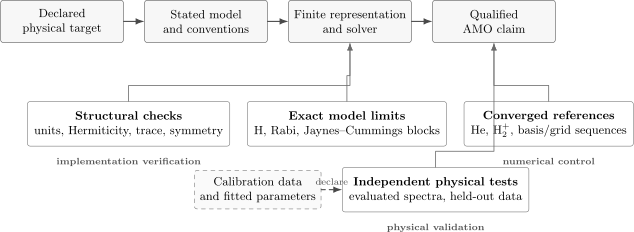
The AMO evidence ladder. Structural checks and exact model limits verify an implementation; refinement and independent reference values control the finite calculation; held-out data test whether the physical model is adequate for the intended claim. Calibration enters from the side and must be declared before a comparison is called predictive.

A benchmark is a specification

A benchmark needs more than a target number. It should state:

1. the Hamiltonian or equations;
2. units and constants;
3. boundary and initial conditions;
4. basis, grid, or truncation sequence;
5. the observable and normalization;
6. a reference value with provenance;
7. an acceptance metric and tolerance;
8. expected convergence behavior;
9. known failure modes;
10. the software and hardware information relevant to reproducibility.

Without these fields, two correct implementations can appear to disagree because they solved different problems.

Residual and observable tests

For a normalized approximate eigenpair,

$$r = H_N\widetilde c - \widetilde E\widetilde c.$$

A scale-aware residual is

$$\eta_r = \frac{ \lVert r\rVert }{ \lVert H_N\rVert\lVert\widetilde c\rVert + |\widetilde E| \lVert\widetilde c\rVert }.$$

A small $\eta_r$ verifies the finite eigenproblem. It does not establish basis convergence. Observable comparisons should use a declared metric, for example

$$\varepsilon_{\mathrm{rel}} = \frac{ |\widehat O-O_{\mathrm{ref}}| }{ \max \left( |O_{\mathrm{ref}}|, O_{\mathrm{scale}} \right) }.$$

The scale floor $O_{\mathrm{scale}}$ prevents a meaningless relative error near a true zero. Symmetry-forbidden matrix elements are better tested with an absolute tolerance tied to operator and state norms.

Atomic Benchmarks

Atomic calculations provide a progression from analytic one-electron tests to correlated and relativistic many-electron structure.

Hydrogenic radial equation

For a central potential, write

$$\psi_{nlm}(\mathbf r) = \frac{u_{nl}(r)}{r} Y_{lm}(\theta,\phi).$$

In atomic units, the radial Coulomb equation is

$$\left[ -\frac{1}{2} \frac{d^2}{dr^2} + \frac{l(l+1)}{2r^2} - \frac{Z}{r} \right] u_{nl}(r) = E_n u_{nl}(r),$$

with

$$u_{nl}(0)=0, \qquad u_{nl}(r)\to0 \quad \text{as } r\to\infty.$$

A radial solver should test:

• the $-Z^2/(2n^2)$ energy sequence;
• normalization $\int_0^\infty |u_{nl}(r)|^2\,dr=1$;
• node count $n-l-1$;
• near-origin behavior $u_{nl}\propto r^{l+1}$;
• exponential tail behavior;
• degeneracy in $l$ for the pure Coulomb Hamiltonian;
• the Coulomb virial identity $2\langle T\rangle+\langle V\rangle=0$;
• convergence with grid spacing, outer radius, and origin treatment.

Hydrogen reveals several common bugs at once: a missing radial Jacobian, an incorrect centrifugal factor, an origin singularity, a wrong sign in the potential, or normalization with Cartesian rather than radial weights.

Helium as a correlation benchmark

For an infinitely massive nucleus in atomic units,

$$H = \sum_{i=1}^{2} \left( -\frac{1}{2}\nabla_i^2 - \frac{2}{r_i} \right) + \frac{1}{r_{12}}.$$

Use a normalized product of hydrogenic $1s$ orbitals with variational effective charge $\zeta$. Its energy is

$$E(\zeta) = \zeta^2 - \frac{27}{8}\zeta.$$

Stationarity gives

$$\zeta_\star = \frac{27}{16}, \qquad E(\zeta_\star) = -\frac{729}{256} E_{\mathrm h} = -2.84765625 E_{\mathrm h}.$$

This small calculation is useful because every integral is analytic, the variational inequality is known, and the remaining discrepancy has a clear physical interpretation: a single uncorrelated spatial product cannot adapt explicitly to the instantaneous electron–electron separation.

High-precision explicitly correlated calculations give a nonrelativistic infinite-mass ground-state reference near

$$E_0 \approx -2.9037243770341196 E_{\mathrm h}.$$

The value is a benchmark for that Hamiltonian, not a prediction including finite nuclear mass, relativity, or QED. Helium Atom owns the physical derivation and correlation interpretation.

Central-field and many-electron checks

For self-consistent atomic structure, useful checks include:

• one-electron ions, where electron–electron terms must vanish;
• two-electron closed shells, where restricted formulas are transparent;
• invariance under rotations within a fully occupied orbital subspace;
• orthonormality of orbitals;
• self-consistency residuals;
• total-energy stationarity;
• term, parity, and total-angular-momentum labels;
• agreement between length and velocity forms of transition amplitudes as a diagnostic, with due care about model consistency;
• convergence in radial grid, orbital set, configuration space, and partial waves.

Length–velocity agreement is not a theorem that the answer is physically exact. Two forms can agree because they share an approximation, and they can disagree when basis completeness or Hamiltonian consistency is insufficient.

Comparison with evaluated spectra

The NIST Atomic Spectra Database provides critically compiled atomic levels, wavelengths, and transition data. A responsible comparison records:

• database version or access date;
• species, ionization stage, isotope when relevant, and level labels;
• observed versus Ritz value;
• vacuum versus standard-air wavelength convention;
• uncertainty and accuracy code;
• whether the entry is experimental, theoretical, or derived;
• the original source cited by the database.

Evaluated data validate a physical prediction only when the calculation and entry refer to the same quantity. Agreement of a nonrelativistic energy with a measured line can be accidental if omitted corrections cancel.

Atomic benchmark ladder

Level	Problem	Primary test	What it does not prove
A0	hydrogenic matrix elements	analytic integrals and selection-rule zeros	many-electron correctness
A1	hydrogen radial spectrum	energy, nodes, virial theorem, refinement	relativistic accuracy
A2	helium effective-charge trial	analytic energy and variational bound	correlation completeness
A3	high-precision helium	basis and correlation convergence	finite-mass or QED accuracy
A4	selected multi-electron atom	term labels, transitions, cross-method comparison	transferability to all atoms
A5	evaluated spectral data	uncertainty-aware physical comparison	predictive status if fitted

Molecular Benchmarks

Molecular computation adds moving nuclei, geometry, nonorthogonal basis functions, multiple electronic structures, and observables obtained from derivatives of an energy surface.

The generalized eigenproblem

For basis functions $|\chi_\mu\rangle$ that are not orthonormal,

$$|\phi_i\rangle = \sum_\mu C_{\mu i} |\chi_\mu\rangle.$$

Projection gives

$$FC = SC\varepsilon,$$

where

$$F_{\mu\nu} = \langle\chi_\mu|\widehat F|\chi_\nu\rangle, \qquad S_{\mu\nu} = \langle\chi_\mu|\chi_\nu\rangle.$$

The metric normalization is

$$C^\dagger S C = I.$$

A solver must not silently treat $S$ as the identity. Small eigenvalues of $S$ signal near-linear dependence and can amplify roundoff. Removing directions requires a documented threshold and a test of observable sensitivity.

Hydrogen molecular ion

The one-electron ion $\mathrm{H}_2^+$ is the molecular analogue of the hydrogen benchmark. For fixed internuclear separation $R$,

$$H_{\mathrm e}(R) = -\frac{1}{2}\nabla^2 - \frac{1}{r_A} - \frac{1}{r_B} + \frac{1}{R}.$$

It tests:

• two-center integrals;
• overlap and generalized diagonalization;
• gerade and ungerade symmetry;
• bonding and antibonding combinations;
• the dissociation and united-atom limits;
• the shape and minimum of a potential-energy curve;
• interpolation and differentiation of that curve.

At large $R$, the electronic state should approach a hydrogen atom plus a proton, with the chosen energy zero stated. At $R\to0$, the electronic part approaches the united-atom problem while the nuclear repulsion diverges. These limits catch energy-zero and nuclear-repulsion bookkeeping errors.

Basis and method are independent axes

A molecular result depends on both the electronic-structure approximation $M$ and finite basis $X$:

$$E_{M,X}.$$

A basis sequence at fixed method estimates

$$\delta_{\mathrm{basis}} \sim E_{M,X} - E_{M,\infty},$$

while a method sequence at a large basis probes a different error:

$$\delta_{\mathrm{method}} \sim E_{M,\infty} - E_{\mathrm{exact},\infty}.$$

Increasing basis size does not turn Hartree–Fock into a correlated method. Increasing correlation rank in a poor basis does not reach the complete-basis result. Report both axes.

Size consistency and dissociation

For noninteracting fragments at infinite separation, a size-consistent method should satisfy

$$E(A+B) \longrightarrow E(A)+E(B).$$

Truncated configuration interaction can violate this property even when its energy is variational. Restricted single-reference methods can also give a qualitatively wrong dissociation curve when one determinant ceases to describe the separated fragments.

The lesson is broader than one method: a near-equilibrium energy benchmark does not validate bond breaking, excited states, charge transfer, or multireference regions.

Basis-set superposition

In a dimer calculation, each fragment can borrow basis functions centered on the other fragment. The raw interaction energy

$$\Delta E_{\mathrm{int}} = E_{AB}^{AB} - E_A^A - E_B^B$$

then compares calculations in unequal one-particle spaces. A counterpoise comparison instead evaluates monomers in the dimer basis:

$$\Delta E_{\mathrm{int}}^{\mathrm{CP}} = E_{AB}^{AB} - E_A^{AB} - E_B^{AB}.$$

Counterpoise correction is a diagnostic and convention that must be reported, not a universal substitute for basis convergence.

Vibrational benchmarks

Near a stationary geometry, expand the potential:

$$V(\mathbf R_0+\Delta\mathbf R) \approx V(\mathbf R_0) + \frac{1}{2} \Delta\mathbf R^{\mathsf T} K \Delta\mathbf R.$$

The mass-weighted Hessian is

$$D_{A\alpha,B\beta} = \frac{ K_{A\alpha,B\beta} }{ \sqrt{M_A M_B} }.$$

Its positive nonzero eigenvalues are $\omega_k^2$ in the harmonic approximation. A molecular-vibration implementation should check:

• translational and rotational zero modes;
• invariance under rigid translation and rotation;
• Hessian symmetry;
• finite-difference step convergence when derivatives are numerical;
• unit conversion from angular frequency to wavenumber;
• analytic oscillator cases;
• sensitivity to geometry and electronic-structure method.

Imaginary frequencies can identify a saddle point, but they can also result from an unconverged geometry, insufficient integration grid, noisy finite differences, or inconsistent constraints.

Molecular benchmark ladder

Level	Problem	Primary test	Failure exposed
M0	overlap matrix	Hermiticity, positive definiteness, metric normalization	basis indexing and linear dependence
M1	$\mathrm{H}_2^+$ minimal basis	analytic or reference integrals, symmetry, limits	generalized-eigenproblem errors
M2	$\mathrm{H}_2^+$ basis sequence	variational energy curve and equilibrium	basis incompleteness
M3	helium or $\mathrm{H}_2$ correlation sequence	method and basis axes	missing dynamical correlation
M4	stretched bond	dissociation and size consistency	single-reference failure
M5	harmonic molecule	zero modes and Hessian convergence	geometry, derivative, and unit errors
M6	held-out spectroscopy	frequencies, isotope trends, uncertainty	physical model inadequacy

Quantum-Optical Simulations

Quantum optics supplies small models with strong analytic structure and large models where truncation and open-system dynamics become decisive.

Closed two-level dynamics

For a time-independent finite Hermitian Hamiltonian,

$$U(t) = \exp \left( -\frac{iHt}{\hbar} \right)$$

is unitary. A propagation benchmark should test:

$$U^\dagger U = I, \qquad \lVert\psi(t)\rVert = 1, \qquad \langle H\rangle_t = \langle H\rangle_0.$$

The last identity applies only when $H$ is time independent. For a driven Hamiltonian, energy exchange with the drive is expected, while norm conservation remains.

Rabi oscillations test frequency, phase, detuning, pulse area, and basis ordering. Useful cases include:

• zero coupling, where populations remain fixed;
• resonance, where a $\pi$ pulse inverts the ideal system;
• large detuning, where excitation is suppressed;
• a drive phase change, which rotates the Bloch-sphere axis;
• comparison of rotating-wave and full driven Hamiltonians.

Optical Bloch steady state

Let $\Gamma_1$ be population decay and $\Gamma_2$ coherence decay. With Rabi frequency convention

$$H_{\mathrm{rot}} = -\frac{\hbar\Delta}{2}\sigma_z + \frac{\hbar\Omega}{2}\sigma_x,$$

the steady excited-state population can be written

$$\rho_{ee}^{(\mathrm{ss})} = \frac{s}{2(1+s)},$$

where

$$s = \frac{ \Omega^2\Gamma_2 }{ \Gamma_1 \left( \Delta^2+\Gamma_2^2 \right) }.$$

For pure radiative broadening, $\Gamma_2=\Gamma_1/2$. This benchmark tests detuning signs, factors of two in the drive, decay conventions, and the saturation limit

$$\rho_{ee}^{(\mathrm{ss})} \longrightarrow \frac{1}{2}.$$

Optical Bloch Equations owns the physical derivation.

Master-equation structure

A Lindblad-form model is

$$\dot\rho = -\frac{i}{\hbar} [H,\rho] + \sum_k \left( L_k\rho L_k^\dagger - \frac{1}{2} \left\{ L_k^\dagger L_k, \rho \right\} \right).$$

The represented evolution should preserve trace and Hermiticity and, for a valid implementation of the stated generator, positivity. Numerical checks include:

$$\left| \operatorname{Tr}\rho-1 \right|, \qquad \lVert\rho-\rho^\dagger\rVert, \qquad \min_j\lambda_j(\rho).$$

A tiny negative eigenvalue can be roundoff; a persistent negative population can indicate an integrator, generator, or approximation problem. Clipping negative eigenvalues hides the symptom and changes the dynamics.

Quantum trajectories

An unraveling estimates the density operator by an ensemble:

$$\rho(t) \approx \frac{1}{M} \sum_{j=1}^{M} |\psi_j(t)\rangle \langle\psi_j(t)|.$$

The ensemble mean should converge to the master-equation result for the same generator. This cross-method comparison is stronger than either solver alone. Report confidence intervals and compare multiple seeds; individual trajectories are not expected to match deterministic density-matrix curves.

Jaynes–Cummings blocks

For

$$H = \hbar\omega_c a^\dagger a + \frac{\hbar\omega_a}{2}\sigma_z + \hbar g \left( a^\dagger\sigma_- + a\sigma_+ \right),$$

the excitation number

$$N_{\mathrm{exc}} = a^\dagger a + \sigma_+\sigma_-$$

is conserved. In the manifold $\{|e,n\rangle,|g,n+1\rangle\}$,

$$E_{n,\pm} = \hbar\omega_c \left( n+\frac{1}{2} \right) \pm \frac{\hbar}{2} \sqrt{ \Delta^2 + 4g^2(n+1) }.$$

At resonance, the splitting is

$$E_{n,+}-E_{n,-} = 2\hbar g\sqrt{n+1}.$$

This gives an exact finite-block benchmark for matrix construction. A full-space simulation still needs a photon cutoff. Convergence should be checked through both observables and the occupation near the highest retained number state.

Quantum-optical benchmark ladder

Level	Benchmark	Required evidence
Q0	Pauli and ladder-operator matrices	commutators, dimensions, basis ordering
Q1	undriven two-level propagator	phase and norm
Q2	Rabi formula	amplitude, generalized frequency, pulse area
Q3	optical Bloch steady state	trace, positivity, saturation, detuning
Q4	Jaynes–Cummings block	conserved excitation and analytic doublet
Q5	photon-cutoff sequence	tail occupation and observable stability
Q6	trajectories versus master equation	confidence-aware ensemble agreement

AMO Platform Simulations

Platform calculations combine internal quantum dynamics with motion, electromagnetic fields, geometry, feedback, and noise. Their outputs are often effective parameters or measured signals rather than bare eigenvalues.

Low-saturation Doppler force

For two counterpropagating beams of equal low saturation $s_0\ll1$, a simple one-dimensional force model is

$$\begin{aligned} F(v) = \frac{\hbar k\Gamma s_0}{2} \Bigg[ & \frac{1}{ 1+4(\Delta-kv)^2/\Gamma^2 } \\ - & \frac{1}{ 1+4(\Delta+kv)^2/\Gamma^2 } \Bigg]. \end{aligned}$$

For red detuning $\Delta<0$, the small-velocity slope should oppose motion:

$$F(v) \approx -\alpha v, \qquad \alpha>0.$$

This benchmark catches beam-direction, Doppler-shift, detuning, and recoil sign errors. It does not validate a sub-Doppler, multilevel, polarization gradient, or high-saturation model.

Separate internal and motional approximations

A semiclassical simulation may evolve

$$m\ddot{\mathbf r} = \mathbf F \left( \mathbf r, \mathbf v, \rho, t \right) + \boldsymbol\xi(t)$$

while a master equation evolves the internal state $\rho$. The assumptions behind classical motion, local steady state, recoil diffusion, and white noise are independent. State them separately.

For a stochastic recoil model, checks include:

• zero mean recoil in an isotropic emission model;
• the expected momentum-diffusion growth;
• convergence in trajectory count and time step;
• detailed treatment of absorption and emission directions;
• consistency between friction and diffusion in the regime where an equilibrium temperature is inferred.

Traps and fields

Near a stable trap center,

$$V(\mathbf r) \approx V_0 + \frac{m}{2} \sum_i \omega_i^2 x_i^2.$$

A field or trajectory solver should test:

• Maxwell constraints appropriate to the field representation;
• symmetry points and known zero-field or zero-force locations;
• Hessian eigenvalues and trap frequencies;
• energy conservation for static conservative motion;
• secular-frequency limits for driven traps;
• convergence in mesh, multipole order, and integration step;
• sensitivity to electrode, beam, and alignment parameters.

The trap depth, harmonic frequency, scattering rate, and coherence time are different observables and need not converge at the same rate.

Cavity and circuit platforms

An effective cavity simulation should declare:

• retained matter levels and modes;
• coupling convention and mode normalization;
• detuning and rotating frame;
• coherent drives;
• cavity loss, matter decay, and dephasing channels;
• input–output normalization;
• photon cutoff;
• initial state and measurement operator.

Strong coupling is an observable-dependent comparison among $g$, decay rates, dephasing, detuning, and spectral resolution. Reproducing an avoided crossing in a closed Jaynes–Cummings matrix does not by itself predict a measurable split transmission line.

Control sequences

For pulses, retain the full envelope and phase convention:

$$\Omega(t) = \frac{ \mathbf d\cdot\mathbf E_0(t) }{ \hbar } e^{i\phi(t)}.$$

Report whether $\Omega$ is a signed, complex, peak, or root-mean-square quantity. Pulse-area agreement,

$$\Theta = \int \Omega(t)\,dt,$$

is a useful ideal benchmark but does not guarantee equal dynamics under detuning, bandwidth, leakage, Stark shifts, or decoherence.

Platform benchmark ladder

Level	Benchmark	Main check
P0	zero field or zero drive	no spurious force or transition
P1	harmonic trap	analytic frequency and conserved energy
P2	low-saturation two-beam force	oddness in $v$ and red-detuned damping
P3	ideal pulse sequence	pulse area, phase, and frame convention
P4	recoil ensemble	mean, variance, seed, and time-step convergence
P5	measured calibration curve	held-out parameters and uncertainty

Designing a Benchmark Suite

A mature suite should contain complementary tests rather than one flagship number.

Structural tests

Run on every change:

• dimensions and units;
• Hermiticity or symmetry;
• normalization and trace;
• basis ordering;
• selection-rule zeros;
• conserved quantities;
• exact matrix identities;
• deterministic tiny cases.

These tests are fast and localize implementation regressions.

Convergence tests

Run over explicit sequences:

$$\left\{ N_{\mathrm{basis}}, h, R_{\max}, \Delta t, N_{\mathrm{ph}}, M_{\mathrm{traj}} \right\}.$$

Change one control at a time unless a coupled refinement path is theoretically required. Preserve the raw sequence, not only an extrapolated final value.

For algebraic convergence, report residuals. For discretization, report observed order when an asymptotic regime exists:

$$p_{\mathrm{obs}} \approx \frac{ \log \left( |O_h-O_{h/2}| / |O_{h/2}-O_{h/4}| \right) }{ \log 2 }.$$

A plausible $p_{\mathrm{obs}}$ is evidence that the intended error regime has been reached. It is not a substitute for a continuum or reference comparison.

Cross-formulation tests

Use independent routes where possible:

• radial shooting versus matrix diagonalization;
• real-space versus basis-set hydrogen;
• analytic versus numerical integrals;
• length versus velocity transition forms;
• finite difference versus automatic or analytic derivatives;
• density-matrix versus trajectory dynamics;
• direct steady-state solve versus long-time propagation;
• time-domain spectrum versus resolvent or eigenmode spectrum;
• two independent software implementations.

Independence matters. Two wrappers around the same library do not provide a strong cross-code test.

Physical limit tests

Every model has simplifying limits:

$$\begin{gathered} g\to0, \qquad \Omega\to0, \qquad \Gamma\to0, \qquad R\to\infty, \\ m_N\to\infty, \qquad Z\alpha\to0, \qquad s_0\to0. \end{gathered}$$

The output should approach the correct reduced model. A limit test is often more diagnostic than agreement at one generic parameter point.

Held-out physical tests

If parameters are calibrated on one subset of observations, reserve another subset for validation. Examples include:

• fit an effective quantum defect to some Rydberg levels and predict others;
• fit a molecular potential near equilibrium and test isotope-dependent vibrational spacings;
• calibrate a Rabi frequency at one intensity and test pulse-area scaling;
• calibrate trap frequencies and predict anharmonic shifts;
• fit decay rates and test two-time correlations.

Document the split before inspecting the held-out result whenever a strong predictive claim is intended.

Reproducibility Rules

Reproducibility is the ability to reconstruct the computational argument from preserved inputs, code, environment, and outputs. It is necessary but not sufficient for correctness.

Minimum calculation manifest

Every published calculation should preserve:

Field	Required content
identity	title, author or maintainer, date, artifact version
physical target	species, state, geometry, observable, intended claim
equations	Hamiltonian or generator with conventions
approximations	explicit retained and omitted physics
representation	basis, grid, domain, ordering, truncations
parameters	values, units, constants release, data provenance
algorithm	solver, tolerances, stopping criteria, initialization
environment	language, package versions, lockfile or container recipe
stochastic state	generator, seed policy, ensemble size
benchmark	target, metric, tolerance, pass or fail
outputs	machine-readable data, plots derived from those data
limitations	known failure regimes and unresolved discrepancies

The Environments, Code Style, and Validation Tests pages own the site-wide implementation details.

Units are data

Store values with explicit unit metadata. “Frequency = 10” is incomplete. Even “10 MHz” may be ambiguous if a code expects angular frequency. Use a declared mapping such as

$$\omega = 2\pi \left( 10\,\mathrm{MHz} \right)$$

when the solver parameter is angular frequency. Atomic units should identify the nuclear-mass convention and any conversion constants used.

Geometry and basis are data

A quantum-chemistry method name does not reproduce a calculation. Preserve:

• all nuclear coordinates, units, isotope masses, charge, and multiplicity;
• basis-set name and exact revision or machine-readable basis definition;
• effective core potentials and auxiliary bases;
• frozen-core and active-space choices;
• integration-grid and SCF settings;
• symmetry handling and occupation constraints;
• counterpoise or fragment conventions;
• derivative and geometry-convergence thresholds.

Package defaults are versioned implementation choices, not universal physical conventions.

Preserve the full convergence record

Do not publish only the preferred basis, grid, or cutoff. A convergence table should include:

$$\left( \lambda_j, O_j, r_j, t_j, \text{status}_j \right),$$

where $\lambda_j$ is the refinement control, $O_j$ the observable, $r_j$ a residual or diagnostic, $t_j$ optional resource information, and $\text{status}_j$ any warning or failure.

Failed points are scientifically useful. Removing them can hide instability or a restricted convergence regime.

Separate notebook narrative from reusable computation

A notebook should explain and inspect a calculation. Reusable numerical kernels, parameter validation, and benchmark assertions should live in importable modules or scripts when the calculation grows beyond a small pedagogical example. The notebook should run from a clean state in a declared order and should not depend on invisible interactive variables.

Preserve source data for every figure

A plot is a view, not the primary result. Preserve:

• the machine-readable arrays;
• the script or notebook that produced the plot;
• axis units and transformations;
• fit model and weights;
• uncertainty or confidence data;
• any smoothing, broadening, interpolation, or windowing.

A displayed Lorentzian broadening parameter is part of the result and must not be omitted from provenance.

Deterministic and statistical reproducibility

Bitwise identity can depend on hardware, compiler, thread scheduling, and linear-algebra libraries. The scientific target is often stronger in one sense and weaker in another: independently reproduced observables should agree within a physically and numerically justified tolerance.

For stochastic work, preserve:

• pseudorandom generator family;
• base seed and stream construction;
• number of trajectories or samples;
• aggregation order when numerically relevant;
• uncertainty estimator;
• convergence across independent seed ensembles.

One fixed seed is a regression case, not an uncertainty analysis.

Version benchmarks and tolerances

A benchmark record should have its own version. Change it when:

• the mathematical specification changes;
• constants or reference data change;
• an accepted tolerance changes;
• the intended physical regime changes;
• a bug invalidates prior outputs.

Do not loosen a tolerance merely because a new implementation fails. First determine whether the old tolerance represented theory, observed numerical behavior, or accidental platform-specific digits.

Reproducibility status

Use status labels honestly:

• conceptual: equations and expected behavior are documented;
• implemented: code exists and runs in a declared environment;
• verified: structural and exact-model tests pass;
• converged: numerical controls meet predeclared criteria;
• validated: relevant independent physical comparisons pass;
• archived: code, environment, data, and provenance are preserved.

The Reproducibility Status page owns the global promotion rules. A page should not imply that a planned notebook is already an executable artifact.

A Common AMO Benchmark Record

A compact benchmark report can be organized as

$$\mathcal R = \left( \mathcal P, \mathcal E, \mathcal C, \mathcal V, \mathcal U \right),$$

where:

• $\mathcal P$ is the physical problem declaration;
• $\mathcal E$ is the executable environment;
• $\mathcal C$ is the convergence record;
• $\mathcal V$ is the verification and validation evidence;
• $\mathcal U$ is the uncertainty and limitation statement.

The report should answer five audit questions:

1. Identity: What exact problem was solved?
2. Traceability: Where did every parameter and datum come from?
3. Control: Which errors were varied, bounded, or estimated?
4. Independence: Which checks did not reuse the implementation or data under test?
5. Scope: What claim is supported, and which stronger claims are not?

Chapter Map

The chapter is built as a sequence of domain-specific guides and benchmark notebooks. Titles without links are planned pages rather than published artifacts.

Page	Canonical responsibility	Anchor benchmark
Computational Atomic Structure	method map from radial models through correlation and relativistic corrections	hydrogen and helium
Radial Schrödinger Solvers	boundary conditions, shooting, finite differences, and Numerov-style propagation	hydrogenic spectrum
Variational Helium Notebook	effective-charge trial state and explicit correlation deficit	variational upper bound
Hartree–Fock Notebook	analytic Gaussian integrals, Fock construction, SCF iteration, and convergence separation	closed-shell helium
Molecular Orbital Computation	overlap, generalized eigenproblems, bonding and antibonding orbitals	$\mathrm{H}_2^+$
Electronic Structure Methods Map	responsible choice among HF, DFT, CI, coupled cluster, multireference, and Monte Carlo	method–basis grid
Vibrational Spectra Computation	calibrated mass-weighted Hessian, sinc-DVR Morse levels, transition moments, and experiment-facing error ledger	CO$_2$ stretches and H$^{35}$Cl
Time-Dependent Two-Level Systems Notebook	Rabi, detuning, pulse area, Ramsey, and rotating-wave comparison	analytic Rabi solution
Optical Bloch Equation Notebook	saturation, linewidth, fluorescence, and steady state	analytic steady population
Cavity QED Simulation Notebook	photon cutoff, dressed levels, vacuum Rabi dynamics, coherent-state revival, and optional loss	Jaynes–Cummings doublets
Laser Cooling Simulation Notebook	force curves, friction, recoil diffusion, Doppler temperature, intensity tradeoffs, and relaxation	low-saturation Doppler force
Reproducibility Benchmarks	versioned acceptance suite and expected outputs	complete cross-domain ladder

Suggested routes

For atomic structure, begin with Hydrogen as Atomic Prototype, Helium Atom, and Hartree–Fock for Atoms.

For quantum chemistry, begin with Molecular Hamiltonian, Potential-Energy Surfaces, and Electronic Structure Overview.

For quantum optics, begin with Two-Level Atom, Optical Bloch Equations, and Jaynes–Cummings Model.

For platform simulation, begin with Laser Cooling, Cavity QED Platforms, and Quantum Control in AMO.

Common Mistakes

Calling a converged solver a converged calculation

An eigensolver residual or SCF threshold controls only one layer. Basis, domain, cutoff, model, and parameter errors remain.

Calling a finite matrix exact without qualification

The matrix may be diagonalized accurately while representing the continuum poorly. State “exact diagonalization of the stated finite matrix,” not “exact solution of the atom.”

Benchmarking only total energy

Transition energies, forces, dipoles, polarizabilities, line strengths, and decay rates can converge differently. Test the observable being claimed.

Comparing unlike Hamiltonians

Infinite versus finite nuclear mass, clamped versus vibrating nuclei, nonrelativistic versus relativistic theory, and bare versus effective Hamiltonians produce different reference values.

Hiding defaults

SCF thresholds, integration grids, basis pruning, ODE tolerances, photon cutoffs, and line broadening can change with package versions. Record them.

Using experiment as both fit and prediction

Reproducing fitted data is calibration. Reserve independent data or make a more limited claim.

Treating more digits as more physics

Printed precision can exceed model accuracy, input precision, or experimental meaning. Report uncertainty and scope.

Ignoring nonorthogonal metrics

Molecular orbitals in an atomic basis satisfy $C^\dagger S C=I$, not $C^\dagger C=I$. Ignoring $S$ corrupts energies, populations, and orthogonality.

Clipping unphysical density matrices

Replacing negative eigenvalues by zero can conceal a bad integrator or invalid generator. Diagnose the source before applying any projection.

Checking a cutoff with population alone

A small occupation in the highest photon state is helpful but not sufficient. Observables, transients, and neighboring cutoffs must also be stable.

Confusing reproducibility with correctness

A fully archived notebook can reproducibly implement a sign error. Independent verification and physical validation remain necessary.

Treating a package as a method

A package can implement many Hamiltonians, basis conventions, and algorithms. Scientific claims should name the model and method before the software.

Exercises

1. Classify four exactness claims

Classify each statement and give the missing qualification:

1. “The hydrogen ground-state energy is exact.”
2. “Dense diagonalization gives the exact molecular energy.”
3. “The helium value is exact to fifteen digits.”
4. “The Rabi curve is exact.”

Solution

1. The value $-Z^2E_{\mathrm h}/2$ is analytically exact for the specified nonrelativistic Coulomb Hamiltonian, nuclear-mass convention, and energy zero. It is not the complete physical energy of a real hydrogenic atom.
2. Dense diagonalization can solve a specified finite matrix to floating-point accuracy. The molecular model, one-particle basis, active space, and correlation approximation remain finite or approximate.
3. A high-precision helium value is a numerically converged reference for a stated Hamiltonian. The digits require an uncertainty and convergence argument; finite-mass, relativistic, and QED terms are separate.
4. The Rabi curve is exact for a declared effective two-level Hamiltonian and pulse convention. Level truncation, classical driving, rotating-wave treatment, and absence of decoherence are model assumptions.

The common repair is to say exact for what mathematical object and under which physical assumptions.

2. Separate hydrogen solver errors

A radial finite-difference calculation gives $E_{1s}=-0.4999999999E_{\mathrm h}$ with eigenpair residual $10^{-13}$. List four additional checks needed before claiming a ten-digit continuum result.

Solution

The residual verifies the finite matrix, not the radial continuum problem. Additional checks include:

• refine the radial spacing and establish the expected convergence regime;
• increase the outer boundary and test tail truncation;
• vary the origin treatment and verify $u(r)\propto r$ for $l=0$;
• normalize with the radial measure and verify node count;
• test the virial theorem;
• compare other $n,l$ states rather than only one energy;
• repeat with an independent method such as shooting or a spectral basis.

Ten printed digits in one grid are not a ten-digit error estimate.

3. Derive the helium effective-charge result

For

$$E(\zeta) = \zeta^2 - \frac{27}{8}\zeta,$$

find the stationary point and energy. Explain why the result is an upper bound but not a complete estimate of physical helium.

Solution

Differentiate:

$$\frac{dE}{d\zeta} = 2\zeta - \frac{27}{8}.$$

Thus

$$\zeta_\star = \frac{27}{16}.$$

Substitution gives

$$\begin{aligned} E(\zeta_\star) &= \left( \frac{27}{16} \right)^2 - \frac{27}{8} \left( \frac{27}{16} \right) \\ &= -\frac{729}{256} E_{\mathrm h} \\ &= -2.84765625 E_{\mathrm h}. \end{aligned}$$

The trial state is normalized and belongs to the domain of the stated nonrelativistic infinite-mass Hamiltonian, so Rayleigh–Ritz makes this an upper bound to that model’s ground-state energy. It omits explicit electron–electron correlation through $r_{12}$ and does not include finite nuclear mass, relativistic, radiative, or nuclear-size corrections.

4. Reduce a generalized eigenproblem

Assume $F=F^\dagger$ and $S=S^\dagger>0$. Show how to transform

$$FC = SC\varepsilon$$

into an ordinary Hermitian eigenproblem, and state the numerical warning when $S$ has a very small eigenvalue.

Solution

Because $S$ is positive definite, it has a Hermitian square root. Write

$$S = U s U^\dagger, \qquad S^{-1/2} = U s^{-1/2}U^\dagger.$$

Set

$$C = S^{-1/2}Y.$$

Multiplying on the left by $S^{-1/2}$ gives

$$\left( S^{-1/2}FS^{-1/2} \right) Y = Y\varepsilon.$$

The transformed matrix is Hermitian. If $Y^\dagger Y=I$, then

$$C^\dagger S C = I.$$

A very small eigenvalue of $S$ makes $S^{-1/2}$ large and amplifies roundoff and integral errors. Removing that direction changes the represented space, so the threshold and observable sensitivity must be reported.

5. Check optical Bloch limits

Using

$$\rho_{ee}^{(\mathrm{ss})} = \frac{s}{2(1+s)}, \qquad s = \frac{ \Omega^2\Gamma_2 }{ \Gamma_1 \left( \Delta^2+\Gamma_2^2 \right) },$$

find the weak-drive and strong-drive limits. For pure radiative broadening, write $s$ in terms of $\Gamma_1$.

Solution

For $s\ll1$,

$$\rho_{ee}^{(\mathrm{ss})} \approx \frac{s}{2},$$

so the response is quadratic in the drive amplitude and Lorentzian in detuning. For $s\gg1$,

$$\rho_{ee}^{(\mathrm{ss})} \longrightarrow \frac{1}{2},$$

which is the saturated two-level population.

For pure radiative broadening,

$$\Gamma_2 = \frac{\Gamma_1}{2},$$

and therefore

$$s = \frac{ \Omega^2/2 }{ \Delta^2+\Gamma_1^2/4 } = \frac{ 2\Omega^2 }{ \Gamma_1^2+4\Delta^2 }.$$

This result depends on the stated Hamiltonian and Rabi-frequency convention; it is precisely the kind of factor-of-two benchmark a solver should include.

6. Diagnose a photon cutoff

A cavity simulation with cutoff $n_{\max}=10$ reports $P(n=10)=10^{-9}$ at the final time. Is cutoff convergence established? Design a stronger test.

Solution

No. Final-time boundary population can miss transient occupation, coherences with the boundary, or an observable that is sensitive to a small high-number tail.

A stronger test records the maximum boundary and near-boundary occupation over the full trajectory, then repeats the calculation for a sequence such as $n_{\max}=8,10,12,14$. Compare every claimed observable, trace, positivity, and conservation law where applicable. The cutoff is controlled only when the observables and diagnostics are stable within a predeclared tolerance.

7. Verify the Doppler-force sign

For the low-saturation force on this page, expand to first order in $v$ and show that red detuning produces damping.

Solution

Define

$$f(x) = \frac{1}{ 1+4x^2/\Gamma^2 }.$$

Then

$$F(v) = \frac{\hbar k\Gamma s_0}{2} \left[ f(\Delta-kv) - f(\Delta+kv) \right].$$

For small $v$,

$$f(\Delta\mp kv) \approx f(\Delta) \mp kv f'(\Delta).$$

Hence

$$F(v) \approx -\hbar k^2\Gamma s_0 f'(\Delta)v.$$

Since

$$f'(\Delta) = -\frac{ 8\Delta/\Gamma^2 }{ \left( 1+4\Delta^2/\Gamma^2 \right)^2 },$$

$f'(\Delta)>0$ for $\Delta<0$. Therefore

$$F(v) \approx -\alpha v, \qquad \alpha = \hbar k^2\Gamma s_0 f'(\Delta) >0.$$

This verifies the sign in the low-saturation two-level model, not the validity of that model for multilevel or sub-Doppler cooling.

8. Audit a computational claim

A paper reports a molecular dissociation energy that agrees with experiment to $0.1\%$. It gives the method and basis-set names but no geometries, convergence sequence, relativistic or zero-point treatment, software version, or uncertainty. The same experimental value was used to tune one method parameter. What can be concluded, and what evidence is missing?

Solution

The numerical agreement can be reported, but it is a calibration result rather than an independent prediction because the experimental datum helped tune the method. The comparison also does not reveal whether errors cancel.

Missing evidence includes:

• fragment and molecular geometries, charges, multiplicities, and energy zero;
• electronic versus zero-point-corrected dissociation convention;
• basis and correlation convergence;
• basis-set superposition treatment;
• frozen-core, relativistic, and other corrections;
• solver and geometry thresholds;
• package version and relevant defaults;
• provenance and uncertainty of the experimental value;
• parameter-fit procedure and covariance;
• held-out molecules or observables for validation;
• a complete computational environment and input record.

A defensible claim would identify the result as calibrated, preserve the full calculation, and test transferability on data excluded from the fit.

References

Atomic and numerical structure

• W. R. Johnson, Atomic Structure Theory: Lectures on Atomic Physics, Springer, 2007, doi:10.1007/978-3-540-68013-0.
• I. P. Grant, Relativistic Quantum Theory of Atoms and Molecules: Theory and Computation, Springer, 2007, doi:10.1007/978-0-387-35069-1.
• C. Froese Fischer, G. Tachiev, G. Gaigalas, and M. R. Godefroid, “An MCHF atomic-structure package for large-scale calculations,” Computer Physics Communications 176, 559–579 (2007), doi:10.1016/j.cpc.2007.01.006.
• J. S. Sims and S. A. Hagstrom, “High precision Hy-CI variational calculations for the ground state of neutral helium and helium-like ions,” International Journal of Quantum Chemistry 90 (2002), NIST publication record.
• A. Kramida, Yu. Ralchenko, J. Reader, and the NIST ASD Team, NIST Atomic Spectra Database, National Institute of Standards and Technology, current evaluated release.
• L. N. Trefethen and D. Bau III, Numerical Linear Algebra, SIAM, 1997, doi:10.1137/1.9781611977165.

Quantum chemistry

• T. Helgaker, P. Jørgensen, and J. Olsen, Molecular Electronic-Structure Theory, Wiley, 2000, doi:10.1002/9781119019572.
• A. Szabo and N. S. Ostlund, Modern Quantum Chemistry: Introduction to Advanced Electronic Structure Theory, Dover, 1996.
• C. C. J. Roothaan, “New developments in molecular orbital theory,” Reviews of Modern Physics 23, 69–89 (1951), doi:10.1103/RevModPhys.23.69.
• P. Hohenberg and W. Kohn, “Inhomogeneous electron gas,” Physical Review 136, B864–B871 (1964), doi:10.1103/PhysRev.136.B864.
• W. Kohn and L. J. Sham, “Self-consistent equations including exchange and correlation effects,” Physical Review 140, A1133–A1138 (1965), doi:10.1103/PhysRev.140.A1133.
• K. Raghavachari, G. W. Trucks, J. A. Pople, and M. Head-Gordon, “A fifth-order perturbation comparison of electron correlation theories,” Chemical Physics Letters 157, 479–483 (1989), doi:10.1016/S0009-2614(89)87395-6.
• T. H. Dunning Jr., “Gaussian basis sets for use in correlated molecular calculations. I. The atoms boron through neon and hydrogen,” Journal of Chemical Physics 90, 1007–1023 (1989), doi:10.1063/1.456153.
• T. Helgaker, W. Klopper, H. Koch, and J. Noga, “Basis-set convergence of correlated calculations on water,” Journal of Chemical Physics 106, 9639–9646 (1997), doi:10.1063/1.473863.
• S. F. Boys and F. Bernardi, “The calculation of small molecular interactions by the differences of separate total energies. Some procedures with reduced errors,” Molecular Physics 19, 553–566 (1970), doi:10.1080/00268977000101561.
• D. G. A. Smith et al., “The MolSSI QCArchive project: An open-source platform to compute, organize, and share quantum chemistry data,” WIREs Computational Molecular Science 11, e1491 (2021), doi:10.1002/wcms.1491.

Quantum optics and platform computation

• C. W. Gardiner and P. Zoller, Quantum Noise, 3rd ed., Springer, 2004, doi:10.1007/978-3-662-20907-2.
• H. J. Carmichael, An Open Systems Approach to Quantum Optics, Springer, 1993, doi:10.1007/978-3-540-47620-7.
• J. Dalibard, Y. Castin, and K. Mølmer, “Wave-function approach to dissipative processes in quantum optics,” Physical Review Letters 68, 580–583 (1992), doi:10.1103/PhysRevLett.68.580.
• R. Dum, P. Zoller, and H. Ritsch, “Monte Carlo simulation of the atomic master equation for spontaneous emission,” Physical Review A 45, 4879–4887 (1992), doi:10.1103/PhysRevA.45.4879.
• N. Lambert et al., “QuTiP 5: The Quantum Toolbox in Python,” Physics Reports 1153, 1–62 (2026), doi:10.1016/j.physrep.2025.10.001.
• H. J. Metcalf and P. van der Straten, Laser Cooling and Trapping, Springer, 1999, doi:10.1007/978-1-4612-1470-0.

Reproducibility and evidence

• G. K. Sandve, A. Nekrutenko, J. Taylor, and E. Hovig, “Ten simple rules for reproducible computational research,” PLoS Computational Biology 9, e1003285 (2013), doi:10.1371/journal.pcbi.1003285.
• M. D. Wilkinson et al., “The FAIR Guiding Principles for scientific data management and stewardship,” Scientific Data 3, 160018 (2016), doi:10.1038/sdata.2016.18.
• M. Barker et al., “Introducing the FAIR Principles for research software,” Scientific Data 9, 622 (2022), doi:10.1038/s41597-022-01710-x.

Further Study

• Numerical Mathematics
• Benchmark Problems
• Convergence Tests
• Error Estimates
• Matrix Diagonalization
• ODE Solvers
• Software, Notebooks, and Benchmarks
• Analytic Benchmarks
• Numerical Benchmarks
• Computational Quantum Mechanics Roadmap
• Quantum Chemistry Roadmap
• Computational QM References
• AMO Bibliography and Reading Guide distinguishes method literature, software citations, evaluated data, and reproducibility records.