Radial Schrödinger Solvers

A radial bound-state solver is a boundary-value eigensolver on the half-line. It must find both an energy and a nonzero radial function that is regular at the origin, decays at large radius, has the intended node count, and remains stable under changes of grid, box, propagation direction, and solver tolerance.

The differential equation is short; the evidence chain is not. The most common failures are:

• starting at the singular origin with inconsistent data;
• integrating a forbidden-region growing solution instead of the desired decaying one;
• finding a zero of an unreliable boundary residual;
• resolving the grid while leaving the finite box unconverged;
• confusing a pseudostate with a bound state;
• and validating only the energy while the wavefunction or radial integrals remain inaccurate.

This page develops two complementary routes:

1. shooting and matching, which propagate trial solutions and search for a matching energy;
2. matrix discretization, which converts the radial operator into a finite Hermitian eigenproblem.

Numerov propagation exploits the special second-order structure and can be used in either route. Hydrogenic ions provide an unusually complete benchmark: exact energies, node counts, moments, degeneracies, scaling laws, and wavefunctions.

Canonical Scope

The Radial Schrödinger Equation owns the separation from three dimensions and the relation between $R_\ell(r)$ and $u_\ell(r)$. The Boundary Conditions for Radial Wavefunctions page owns the physical half-line domain and self-adjointness cautions. The ODE Solvers and Finite Difference Methods pages own generic integration and stencil theory.

This page owns their atomic radial specialization:

• asymptotic numerical starting data at both boundaries;
• stable outward and inward propagation;
• two-sided logarithmic-derivative or Wronskian matching;
• Numerov startup, recurrence, and renormalization;
• radial finite-difference Hamiltonians;
• node-aware energy bracketing;
• stitching, normalization, and observable checks;
• and a reproducible hydrogenic benchmark ladder.

The target is a local, energy-independent, single-channel central potential. Nonlocal Hartree–Fock exchange, coupled radial channels, resonances, and continuum scattering require extensions; they are discussed only at the boundary.

Problem Contract

For reduced mass $\mu$, angular momentum $\ell$, and a local central potential $V(r)$, define

$$u_\ell(r)=rR_\ell(r).$$

The reduced radial equation is

$$\left[ -\frac{\hbar^2}{2\mu} \frac{d^2}{dr^2} + \frac{\hbar^2\ell(\ell+1)}{2\mu r^2} +V(r) \right] u_\ell(r) = E u_\ell(r).$$

It is convenient to collect the centrifugal term into

$$V_{\mathrm{eff}}(r) = V(r) + \frac{\hbar^2\ell(\ell+1)}{2\mu r^2}.$$

For a regular bound state in the usual central-potential problem,

$$u_\ell(0)=0, \qquad u_\ell(r)\to0 \quad(r\to\infty),$$

and

$$\int_0^\infty |u_\ell(r)|^2\,dr=1.$$

The normalization measure is $dr$, not $r^2dr$, because the factor of $r$ has already been absorbed into $u$.

Rewrite as a propagation equation

In atomic units with $\mu=1$, write

$$u''(r)=g(r;E)u(r),$$

where

$$g(r;E) = 2\left[V_{\mathrm{eff}}(r)-E\right].$$

The sign of $g$ identifies local behavior:

Region	Sign	Leading behavior
classically allowed	$g<0$	oscillatory
classically forbidden	$g>0$	exponential
turning point	$g=0$	neither local form is uniform

This sign convention must remain consistent with the Numerov recurrence. Many implementation errors arise from copying a formula written for $u''+k^2u=0$ while supplying $g=2(V-E)$.

Inputs and outputs

A solver interface should make the mathematical contract explicit.

Inputs

• potential function and parameter provenance;
• reduced mass and unit system;
• angular momentum $\ell$;
• radial domain and mapping;
• origin and asymptotic boundary models;
• target state or node count;
• energy bracket;
• integration, matrix, and root tolerances.

Outputs

• energy and units;
• normalized $u(r)$ on a stated grid;
• node count and symmetry label;
• boundary and matching residuals;
• normalization and expectation-value checks;
• grid, box, and tolerance convergence tables;
• status flags for failed brackets, overflow, or ambiguous roots.

Returning an energy without diagnostics makes silent misidentification too easy.

Nondimensionalize First

Choose a length scale $a$ and define

$$x=\frac{r}{a}, \qquad \epsilon=\frac{E}{E_a}, \qquad E_a=\frac{\hbar^2}{2\mu a^2}.$$

Then

$$\left[ -\frac{d^2}{dx^2} + \frac{\ell(\ell+1)}{x^2} + v(x) \right]u(x) = \epsilon u(x),$$

with

$$v(x)=\frac{V(ax)}{E_a}.$$

Nondimensionalization keeps matrix entries and residuals near natural scales, clarifies which tolerances are meaningful, and exposes parameter scaling. Atomic units already provide a useful physical nondimensionalization, but a second problem-specific scaling can still help for high-$Z$ ions or diffuse Rydberg states.

For a hydrogenic ion, the change

$$\rho=Zr, \qquad \mathcal E=\frac{E}{Z^2}$$

removes $Z$ from the nonrelativistic radial equation. A correct code should therefore satisfy

$$E_{n\ell}(Z)=Z^2E_{n\ell}(1)$$

after the radial domain and spacing are rescaled consistently.

The Origin Is a Singular Endpoint

The formal boundary condition $u(0)=0$ does not supply two initial values for a second-order propagation. Setting both $u(0)$ and $u'(0)$ to zero produces the trivial solution. Instead, start at a small positive radius $r_{\min}$ using a regular series.

For

$$V(r)=-\frac{Z}{r}+V_0+O(r)$$

and fixed $\ell$, the regular solution has

$$u(r) = A r^{\ell+1} \left[ 1-\frac{Z}{\ell+1}r+O(r^2) \right].$$

The arbitrary constant $A$ fixes only the propagation scale. It disappears from logarithmic derivatives and is replaced by physical normalization after the eigenvalue is found.

Starting values

On a uniform grid $r_j=jh$, a minimal regular startup is

$$\begin{aligned} u_0&=0,\\ u_1&= h^{\ell+1} \left( 1-\frac{Zh}{\ell+1} \right). \end{aligned}$$

For high-order propagation, use enough terms of the local series that startup error is smaller than the interior discretization error. A first-order startup can reduce the observed global order even when the interior Numerov formula is high order.

For large $\ell$, $h^{\ell+1}$ can underflow. Since the equation is linear, rescale the starting pair or initialize logarithmic ratios instead of storing the physical amplitude.

Potentials more singular than Coulomb

If

$$V(r)\sim-\frac{\gamma}{r^p}$$

with $p\ge2$, the regular exponent and even the allowed self-adjoint boundary condition can differ from the Coulomb case. Do not reuse $u\sim r^{\ell+1}$ automatically. Analyze the dominant-balance equation and the operator domain first.

This is not a minor numerical correction: some attractive inverse-square problems require a boundary parameter, and more singular attractive potentials can exhibit collapse without additional short-distance physics.

The Outer Boundary

Suppose

$$V(r)\to V_\infty \qquad(r\to\infty)$$

and $E<V_\infty$. Define

$$\kappa = \frac{\sqrt{2\mu(V_\infty-E)}}{\hbar}.$$

The physical tail decays approximately as

$$u(r)\propto e^{-\kappa r}.$$

If the long-range potential is Coulombic,

$$V(r)\sim-\frac{Q}{r},$$

the leading refinement is

$$u(r)\propto r^{\mu Q/(\hbar^2\kappa)} e^{-\kappa r}.$$

Use this asymptotic form to initialize inward propagation at $R_{\max}$. The overall scale remains arbitrary.

Choosing the box

A bound-state box is adequate only when:

• the wavefunction tail is small at $R_{\max}$;
• the energy and target radial moments are stable as $R_{\max}$ grows;
• the outer boundary lies beyond the relevant turning point;
• and the grid still resolves the larger domain.

Diffuse states are much more demanding than compact ones. For a hydrogenic state, the radial scale grows like

$$r_{\mathrm{typ}}\sim\frac{n^2}{Z}.$$

A box that is excellent for $1s$ can severely distort a Rydberg state.

Box and mesh errors must be separated

At fixed $R_{\max}$, reducing $h$ approaches the eigenproblem in that finite box. At fixed $h$, increasing $R_{\max}$ changes both the number of points and the physical domain. To identify the errors:

1. converge $h$ for several fixed boxes;
2. compare the converged result across boxes;
3. then choose a production pair $(h,R_{\max})$.

A single sequence with constant point count and growing box entangles finer domain coverage with coarser resolution.

Turning Points and Match Radius

A classical turning point satisfies

$$V_{\mathrm{eff}}(r_t)=E.$$

For a typical bound state, outward propagation is well conditioned through the inner allowed region but eventually enters an outer forbidden region. There, any tiny admixture of the growing exponential

$$e^{+\kappa r}$$

will dominate the desired decaying solution. Inward propagation has the opposite advantage: the decaying physical boundary condition can be imposed directly at large radius.

Match the two solutions at a radius $r_m$ in or near the classically allowed region, often close to an outer turning point but away from a node. The result should be stable as $r_m$ is moved within a reasonable interval.

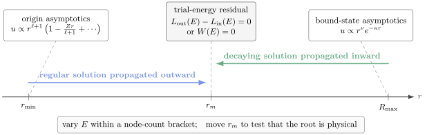
Two-sided shooting suppresses the exponentially unstable direction at each boundary. A trial energy is an eigenvalue when the outward and inward solutions can be rescaled to match both value and derivative at $r_m$. Logarithmic-derivative or Wronskian residuals remove the arbitrary amplitudes.

At a node, $u'/u$ diverges, so move the match point or use a Wronskian residual. A turning point is not a singularity of the exact equation, but a coarse mesh there can degrade matching because the local wavelength changes rapidly.

Shooting as an Eigenvalue Problem

For a trial energy $E$, origin data determine an outward solution $u_{\mathrm{out}}(r;E)$ up to scale. Large-radius asymptotics determine an inward solution $u_{\mathrm{in}}(r;E)$ up to another scale. At an eigenvalue they represent the same global solution.

One-sided endpoint shooting

The simplest residual is

$$F_{\mathrm{end}}(E) = u_{\mathrm{out}}(R_{\max};E).$$

One then searches for

$$F_{\mathrm{end}}(E)=0.$$

This can work for compact low-lying states and moderate boxes. It becomes fragile because the physical forbidden-region solution is the numerically unstable direction under outward propagation. Roundoff and local truncation continually seed the growing exponential.

The sign and magnitude of $u(R_{\max})$ can then be governed more by the arbitrary propagation scale and overflow than by proximity to an eigenvalue. A zero at one box size can move substantially when the box is enlarged.

Use one-sided shooting as a teaching method or a cross-check, not the only evidence for a production radial solver.

Logarithmic-derivative matching

Define

$$L_{\mathrm{out}}(E) = \left. \frac{u_{\mathrm{out}}'}{u_{\mathrm{out}}} \right|_{r_m}, \qquad L_{\mathrm{in}}(E) = \left. \frac{u_{\mathrm{in}}'}{u_{\mathrm{in}}} \right|_{r_m}.$$

The mismatch

$$F_L(E) = L_{\mathrm{out}}(E)-L_{\mathrm{in}}(E)$$

is independent of both arbitrary amplitudes. Eigenvalues satisfy

$$F_L(E)=0.$$

The logarithmic derivative also avoids very large or very small wavefunction amplitudes. Its limitation is a pole whenever the selected match point is a node.

Wronskian matching

An amplitude-independent alternative is the Wronskian

$$\begin{aligned} F_W(E) ={}& W[u_{\mathrm{out}},u_{\mathrm{in}}](r_m) \\ ={}& u_{\mathrm{out}}u_{\mathrm{in}}' -u_{\mathrm{out}}'u_{\mathrm{in}}. \end{aligned}$$

For an exact equation without a first-derivative term, the Wronskian is constant in $r$. It vanishes if and only if the two nonzero solutions are linearly dependent. Numerically, its overall magnitude still scales with the two arbitrary amplitudes, so normalize or rescale the propagated solutions before using it in a root finder.

Wronskian drift across several nearby match points is a useful discretization diagnostic. A root found only at one grid point but not at adjacent points is suspect.

Stitching the state

After finding an eigenvalue, rescale the inward solution by

$$s = \frac{ u_{\mathrm{out}}(r_m) }{ u_{\mathrm{in}}(r_m) }$$

and define

$$u(r) = \begin{cases} u_{\mathrm{out}}(r), & r\le r_m,\\ s\,u_{\mathrm{in}}(r), & r\ge r_m. \end{cases}$$

Then check the derivative mismatch

$$\Delta_m = \frac{ u_{\mathrm{out}}'(r_m) -s\,u_{\mathrm{in}}'(r_m) }{ \max\left( |u_{\mathrm{out}}'(r_m)|, |s\,u_{\mathrm{in}}'(r_m)|, u_{\mathrm{scale}}/r_{\mathrm{scale}} \right) }.$$

The scale floor prevents a meaningless relative blow-up when both derivatives are close to zero. Finally normalize over the entire domain:

$$u(r)\longrightarrow \frac{u(r)}{ \sqrt{\int_0^{R_{\max}}|u(r)|^2\,dr} }.$$

Normalization must follow stitching; normalizing the two halves separately destroys their relative amplitude.

Node Counting and State Identity

For a regular scalar Sturm–Liouville problem, eigenvalues within a fixed $\ell$ sector are ordered by the number of interior nodes. The lowest radial state has no node, the next has one, and so on.

For a hydrogenic state,

$$n_r=n-\ell-1.$$

Thus:

State	$\ell$	Interior radial nodes
$1s$	0	0
$2s$	0	1
$2p$	1	0
$3s$	0	2
$3p$	1	1
$3d$	2	0

Node count protects an energy search from converging to the wrong root. During outward propagation, count sign changes only after suppressing roundoff-scale values and excluding the origin. If a node falls between grid points, interpolate or infer it from a sign-changing bracket.

When node counting needs care

The simple theorem assumes:

• a scalar second-order equation;
• a self-adjoint boundary-value problem;
• a local real potential;
• and a regular ordering within one symmetry sector.

Coupled channels, nonlocal exchange, energy-dependent potentials, and some singular endpoint extensions need generalized methods. A node counter written for the scalar equation should fail explicitly rather than silently assign atomic labels in those settings.

Energy Bracketing

A robust root search begins with a bracket

$$E_{\mathrm L}<E_\nu<E_{\mathrm U}.$$

For a potential tending to zero, bound states require $E<0$. A lower bound can come from a known potential minimum or a comparison potential; an upper bound can lie just below the continuum threshold. Central-field estimates, WKB quantization, or neighboring parameter values can provide tighter initial intervals.

Bracket with nodes and mismatch

Use two pieces of information:

1. the node count identifies the spectral interval;
2. the matching residual locates the root within that interval.

A practical search is:

choose target radial node count n_r
establish an energy interval below the continuum
scan energies coarsely
for each energy:
    propagate the regular solution outward
    count reliable interior nodes
    evaluate a two-sided matching residual
identify an interval containing the desired node branch and a residual root
refine with a bracket-preserving root solver
verify the node count and move the match point

The coarse scan is not wasted work. It reveals residual poles, missed narrow intervals, and state rearrangements that a blind Newton iteration can skip.

Root algorithms

Method	Advantage	Main risk
bisection	guaranteed contraction for a continuous sign-changing residual	linear convergence
secant	derivative-free and faster near a simple root	can leave the bracket
Brent-style hybrid	robust bracket with superlinear steps when useful	still requires a valid continuous bracket
Newton or Cooley correction	rapid near a well-resolved root	derivative/correction failure far from root or near poles

For production, a bracket-preserving hybrid is a strong default. Stop only when both the energy interval and the physical matching residual meet their tolerances. A small energy step alone is insufficient if the residual is flat or ill scaled.

Residual poles are not eigenvalues

The logarithmic mismatch has poles when either propagated solution vanishes at $r_m$. A sign change across a pole can fool a bracketing solver. Detect large residual magnitudes, track the signs of both denominator values, or switch to a scaled Wronskian near the suspected interval.

Moving $r_m$ is a powerful test: an eigenvalue remains fixed within discretization error, while a pole tied to $u(r_m)=0$ moves.

Numerov Propagation

Numerov exploits the absence of a first-derivative term in

$$u''(r)=g(r)u(r).$$

On a uniform grid $r_j=r_0+jh$, Taylor expansion gives the recurrence

$$\begin{aligned} \left( 1-\frac{h^2}{12}g_{j+1} \right)u_{j+1} ={}& 2\left( 1+\frac{5h^2}{12}g_j \right)u_j \\ &- \left( 1-\frac{h^2}{12}g_{j-1} \right)u_{j-1}. \end{aligned}$$

For the radial Schrödinger equation in atomic units,

$$g_j = 2\left[ V(r_j) +\frac{\ell(\ell+1)}{2r_j^2} -E \right].$$

Numerov has a local recurrence defect of order $h^6$ under the usual smoothness assumptions; the accumulated wavefunction error is commonly $O(h^4)$. Eigenvalue convergence depends on startup, boundary matching, potential regularity, and root extraction, so measure the observed order instead of assigning it from the interior formula alone.

Derivation in one line of structure

Let $f=u''=gu$. The centered identity

$$u_{j+1}-2u_j+u_{j-1} = \frac{h^2}{12} \left( f_{j+1}+10f_j+f_{j-1} \right) +O(h^6)$$

becomes the recurrence after substituting $f_j=g_ju_j$ and collecting the $u_{j\pm1}$ terms.

This derivation shows the assumptions:

• a uniform step in the coordinate used by the recurrence;
• sufficient smoothness through the stencil;
• a linear second-order equation;
• and no first-derivative term.

Stable startup

Numerov requires two adjacent values. For outward propagation, obtain them from the origin series. For inward propagation, use the large-$r$ asymptotic form at $R_{\max}$ and $R_{\max}-h$.

Do not generate the second value with a low-order Euler step. That can dominate the global error. If a high-order asymptotic series is unavailable, start farther inside a region where an adaptive high-order first-order-system solver can supply a consistent pair, then switch to Numerov and test the handoff point.

Renormalized recurrence

Define

$$A_j=1-\frac{h^2}{12}g_j, \qquad B_j=2\left(1+\frac{5h^2}{12}g_j\right).$$

The recurrence is

$$A_{j+1}u_{j+1} = B_ju_j-A_{j-1}u_{j-1}.$$

Using the ratio

$$R_j=\frac{u_j}{u_{j-1}}$$

gives

$$R_{j+1} = \frac{ B_j-A_{j-1}/R_j }{ A_{j+1} }.$$

This renormalized form avoids unbounded absolute amplitudes and supports logarithmic-derivative matching. Ratios have poles at nodes, so practical implementations monitor reciprocal ratios or rescale ordinary solution pairs when needed.

An alternative is periodic amplitude rescaling:

$$(u_{j-1},u_j) \longrightarrow \frac{(u_{j-1},u_j)}{ \max(|u_{j-1}|,|u_j|) }.$$

Store the cumulative scale only if an absolute amplitude is needed before final normalization.

Derivatives at the match point

A centered five-point derivative is

$$u_j' \approx \frac{ u_{j-2} -8u_{j-1} +8u_{j+1} -u_{j+2} }{ 12h },$$

with error $O(h^4)$ for a smooth function. The derivative formula should be commensurate with the propagation accuracy. A first-order one-sided difference can dominate an otherwise high-order matching residual.

Near a boundary or a node, use an appropriate one-sided high-order stencil, move the match point, or derive the logarithmic derivative directly from renormalized ratios.

Nonuniform grids

The basic recurrence cannot be applied unchanged on a logarithmic or arbitrary nonuniform mesh. Under a coordinate map $r=r(x)$,

$$\frac{d^2u}{dr^2} = \frac{1}{r'(x)^2} \frac{d^2u}{dx^2} - \frac{r''(x)}{r'(x)^3} \frac{du}{dx}.$$

The transformed equation contains a first derivative. One may:

• use a generalized nonuniform Numerov formula;
• transform the dependent variable to remove the first derivative;
• use finite elements or collocation in the mapped coordinate;
• or integrate the first-order system with an adaptive solver.

Calling a grid “logarithmic” does not specify which transformed operator or quadrature was used.

Where Numerov loses its advantage

Numerov’s formal order can be degraded by:

• discontinuous or nonsmooth potentials;
• a singular origin treated without an asymptotic startup;
• abrupt mesh changes;
• a turning point resolved by too few steps;
• an energy-dependent or nonlocal interaction;
• coupled equations not handled by a matrix generalization;
• and floating-point overflow in forbidden regions.

A lower-order method with controlled adaptivity and correct boundary data can be more trustworthy than an unverified high-order recurrence.

Finite-Difference Hamiltonian

Matrix discretization enforces both boundaries first and solves for several eigenpairs together. On a uniform grid,

$$r_j=jh, \qquad j=0,1,\ldots,N+1, \qquad R_{\max}=(N+1)h,$$

impose

$$u_0=u_{N+1}=0$$

and retain the $N$ interior values. In atomic units,

$$-\frac12u''(r_j) \approx -\frac{ u_{j+1}-2u_j+u_{j-1} }{ 2h^2 }.$$

The tridiagonal Hamiltonian has

$$\begin{aligned} (H_h)_{jj} &= \frac{1}{h^2} +V_{\mathrm{eff}}(r_j), \\ (H_h)_{j,j+1} &= (H_h)_{j+1,j} = -\frac{1}{2h^2}. \end{aligned}$$

No potential is evaluated at $r=0$. Origin regularity enters through the Dirichlet boundary and the reduced radial representation.

What the matrix eigenvalues mean

The finite matrix has $N$ discrete eigenvalues. Negative eigenvalues stable under box growth approximate physical bound states when the continuum threshold is zero. Positive eigenvalues are generally cavity pseudostates: they move as $R_{\max}$ changes and sample the continuum rather than represent isolated bound levels.

A discrete eigenvalue is therefore classified by:

• its sign relative to the physical threshold;
• stability under box enlargement;
• node count and localization;
• amplitude near the outer boundary;
• and continuity under mesh refinement.

Hermiticity

For a real local potential, the standard matrix is real symmetric:

$$H_h^{\mathsf T}=H_h.$$

Use a Hermitian eigensolver. If an implementation produces appreciably complex eigenvalues, the likely causes include an asymmetric boundary row, an incorrect mapped-coordinate discretization, or a nonsymmetric operator assembly.

The generic eigensolver choices are discussed in Sparse Eigensolvers. For a tridiagonal radial matrix, specialized symmetric tridiagonal routines are often simpler and faster than a general sparse package.

Discrete versus physical normalization

A standard eigensolver returns

$$\sum_{j=1}^{N}|v_j|^2=1.$$

The physical radial normalization on a uniform grid is approximately

$$h\sum_{j=1}^{N}|u_j|^2=1.$$

Thus a Euclidean-normalized eigenvector must be divided by $\sqrt h$ before it is interpreted as sampled values of a continuum-normalized radial function, up to the chosen quadrature accuracy. On a nonuniform grid,

$$\sum_j w_j|u_j|^2=1$$

uses quadrature weights $w_j$.

Confusing the two normalizations leaves energies unchanged but corrupts radial matrix elements.

Higher-order stencils

A five-point fourth-order approximation is

$$u''_j \approx \frac{ -u_{j+2} +16u_{j+1} -30u_j +16u_{j-1} -u_{j-2} }{ 12h^2 }.$$

It makes the Hamiltonian pentadiagonal. The first two and last two rows need boundary formulas of compatible order. Using a fourth-order interior stencil with a first-order boundary closure often returns the whole eigenproblem to low-order convergence.

For Coulomb potentials, the solution has a known cusp structure but remains regular in $u$. Observed convergence can nevertheless differ by $\ell$ and state because high derivatives near the origin grow with $Z$.

Do finite-difference energies approach from above?

Do not assume so. A Rayleigh–Ritz basis method has a variational upper-bound property when its integrals are evaluated consistently. A standard finite-difference operator is a discrete approximation, not automatically the projection of the continuum Hamiltonian onto a nested trial space.

Its eigenvalues can approach from above or below depending on the stencil, boundary treatment, and potential. Monotone behavior observed for one state is not a theorem for the implementation.

Matrix Numerov

The Numerov identity can also be assembled as a matrix eigenproblem. Let $\mathbf D$ be the unscaled tridiagonal second-difference matrix with $-2$ on the diagonal and $1$ on adjacent diagonals, and define

$$\mathbf B = \mathbf I+\frac{1}{12}\mathbf D.$$

For

$$\mathbf u''=2(\mathbf V-E\mathbf I)\mathbf u,$$

the Numerov discretization implies

$$\mathbf D\mathbf u = 2h^2\mathbf B (\mathbf V-E\mathbf I)\mathbf u.$$

Equivalently,

$$\left[ -\frac{1}{2h^2}\mathbf B^{-1}\mathbf D +\mathbf V \right]\mathbf u = E\mathbf u.$$

Because $\mathbf B$ and $\mathbf D$ are both functions of the same symmetric second-difference matrix, $\mathbf B^{-1}\mathbf D$ is symmetric in exact arithmetic for the standard boundary setup. Do not form a dense inverse explicitly; use structured solves or an equivalent generalized formulation.

Matrix Numerov can improve accuracy per grid point for smooth problems. It does not remove:

• finite-box error;
• origin startup or boundary-closure questions;
• singular-potential sensitivity;
• conditioning limits;
• or the need to classify positive-energy pseudostates.

Compare against the simpler tridiagonal Hamiltonian before trusting the more elaborate assembly.

Mapped and Adaptive Radial Grids

Uniform grids are transparent but inefficient when a compact core and diffuse tail coexist. A map $r=r(x)$ can distribute points nonuniformly. The physical norm becomes

$$\int_0^{R_{\max}}|u(r)|^2\,dr = \int_{x_{\min}}^{x_{\max}} |u(r(x))|^2r'(x)\,dx.$$

Defining

$$\chi(x) = \sqrt{r'(x)}\,u(r(x))$$

makes the $x$-space norm ordinary:

$$\int|\chi(x)|^2\,dx = \int|u(r)|^2\,dr.$$

The kinetic operator must be transformed consistently with this change of function and measure. Applying a uniform-grid second derivative to samples on a nonuniform $r$ grid generally produces a non-Hermitian and inconsistent operator.

Useful maps include:

• exponential or logarithmic-like maps for resolving a Coulombic core;
• algebraic maps that retain a long diffuse tail;
• piecewise meshes with controlled transition regions;
• finite elements with local polynomial refinement.

Document map parameters as part of the numerical model. “Two thousand radial points” is not reproducible without their locations and quadrature.

Shooting and Matrix Methods Compared

Criterion	Two-sided shooting	Matrix diagonalization
main output	selected eigenvalue and state	several states in one symmetry block
memory	$O(N)$	$O(N)$ for tridiagonal storage, more for wider operators
eigenvalue location	nonlinear scalar root search	algebraic eigensolver
boundary stability	requires inward/outward design	imposed in matrix rows
state identity	node count plus matching branch	eigenvalue order plus node count
continuum	requires scattering normalization or special treatment	finite-box pseudostates appear automatically
nonlocal potential	awkward	natural as a matrix, but often dense
implementation cross-check	propagation residual	algebraic residual

The two approaches have different failure modes. Agreement across converged implementations is much stronger evidence than agreement between two root algorithms wrapped around the same propagation routine.

Which should be the default?

For a single local bound state with known node count, two-sided shooting is fast and interpretable. For many low-lying states, response sums, or nonlocal operators, matrix methods are often preferable. A mature codebase typically keeps both for unit tests and method cross-checks.

Post-Processing the Wavefunction

An accurate eigenvalue does not guarantee an accurate sampled wavefunction. Post-processing must preserve the radial measure, phase convention, and interpolation order.

Phase and normalization

An eigenfunction has arbitrary overall sign. Choose a reproducible convention, such as

$$u(r)>0$$

at the first grid point where its magnitude exceeds a stated threshold. Then normalize with a quadrature rule whose error is smaller than the wavefunction discretization error.

The Numerical Quadrature page owns generic integration rules.

Radial moments

For a normalized reduced radial function,

$$\langle f(r)\rangle = \int_0^\infty |u(r)|^2f(r)\,dr.$$

Important tests include

$$\langle r\rangle, \qquad \left\langle\frac1r\right\rangle, \qquad \langle r^2\rangle.$$

Positive powers emphasize the diffuse tail; inverse powers emphasize the origin and core. Converging both is more informative than checking normalization alone.

Off-diagonal radial integrals

Transition and coupling calculations require integrals such as

$$I_{ab}^{(k)} = \int_0^\infty u_a(r)r^k u_b(r)\,dr.$$

If $u_a$ and $u_b$ live on different grids, interpolate both onto a common quadrature representation or evaluate them through their basis representations. Low-order interpolation can become the dominant error even when each energy is accurate.

An independent differential residual

Evaluate

$$\mathcal R(r) = -\frac12u''(r) +V_{\mathrm{eff}}(r)u(r) -Eu(r)$$

with a derivative formula or collocation grid independent of the one used to solve the problem. Applying the same matrix that produced the eigenvector mostly measures eigensolver tolerance. An independent residual probes representation error more directly.

A scale-aware norm is

$$\eta_{\mathcal R} = \frac{ \left[ \int|\mathcal R(r)|^2\,dr \right]^{1/2} }{ \left[ \int|E\,u(r)|^2\,dr \right]^{1/2} + \left[ \int|V_{\mathrm{eff}}(r)u(r)|^2\,dr \right]^{1/2} +\epsilon_{\mathrm{floor}} }.$$

Inspect the residual as a function of $r$ as well. A small global norm can hide a localized boundary defect.

Hydrogenic Benchmark

For

$$V(r)=-\frac{Z}{r}$$

in atomic units with infinite nuclear mass,

$$E_n=-\frac{Z^2}{2n^2}, \qquad n=1,2,\ldots .$$

The reduced radial functions have the form

$$u_{n\ell}(r) \propto r \left( \frac{2Zr}{n} \right)^\ell e^{-Zr/n} L_{n-\ell-1}^{2\ell+1} \left( \frac{2Zr}{n} \right),$$

with $0\le\ell\le n-1$. This provides exact energies, shapes, nodes, and moments without fitting numerical data.

Anchor values

State	Exact energy $E_h$	Nodes	$\langle r\rangle/a_0$ for $Z=1$
$1s$	$-1/2$	0	$3/2$
$2s$	$-1/8$	1	$6$
$2p$	$-1/8$	0	$5$
$3s$	$-1/18$	2	$27/2$
$3p$	$-1/18$	1	$25/2$
$3d$	$-1/18$	0	$21/2$

The moment formula used here is

$$\langle r\rangle_{n\ell} = \frac{ 3n^2-\ell(\ell+1) }{ 2Z }.$$

Two further exact checks are

$$\left\langle\frac1r\right\rangle = \frac{Z}{n^2}$$

and the virial decomposition

$$\langle T\rangle = \frac{Z^2}{2n^2}, \qquad \langle V\rangle = -\frac{Z^2}{n^2}.$$

Ground-state shape

The normalized $1s$ reduced radial function is

$$u_{10}(r) = 2Z^{3/2}r e^{-Zr}.$$

It tests:

• the $u(0)=0$ boundary;
• the $s$-wave Coulomb cusp;
• exponential tail decay;
• normalization with measure $dr$;
• and radial moments.

A pointwise comparison should exclude a meaningless relative error exactly at the node $u(0)=0$. Use absolute error near zeros and relative error where the reference amplitude is safely nonzero.

Coulomb degeneracy

In the exact nonrelativistic Coulomb problem,

$$E_{n\ell}=E_n$$

for all allowed $\ell$. A radial grid can break this accidental degeneracy because each $\ell$ has different origin behavior and centrifugal structure. The splitting

$$\Delta_{n;\ell\ell'} = E_{n\ell}^{(h)} -E_{n\ell'}^{(h)}$$

is a sensitive cross-channel discretization diagnostic. It should vanish under a balanced refinement.

Do not enforce the degeneracy by averaging the numerical energies; that hides the error being measured.

Scaling with nuclear charge

Run the same dimensionless calculation for several $Z$. After scaling $r\mapsto r/Z$ and $E\mapsto Z^2E$, the results should collapse. Failure can reveal:

• a unit conversion error;
• an unscaled box or step size;
• a hard-coded hydrogen parameter;
• or loss of resolution near the increasingly compact origin.

Reduced mass

For a finite-mass hydrogenic two-body problem, replace the electron mass by

$$\mu = \frac{m_eM}{m_e+M}.$$

Then

$$E_n = -\frac{\mu}{m_e} \frac{Z^2}{2n^2}$$

when energies are expressed in electron-mass atomic units. A benchmark must state whether it uses $\mu=m_e$ or a finite nuclear mass. Comparing a finite-mass numerical result to the infinite-mass analytic value creates a physical offset that mesh refinement cannot remove.

Benchmark Protocol

Use a staged benchmark rather than one final decimal comparison.

Stage 1: Algebraic checks

• verify the sign convention in $g(r;E)$;
• verify matrix symmetry;
• test the Numerov recurrence on a function with known second derivative;
• test quadrature on analytic radial functions;
• and confirm unit conversions.

Stage 2: One state, two methods

Compute hydrogen $1s$ with:

1. two-sided shooting;
2. a tridiagonal finite-difference Hamiltonian.

Compare energy, $\langle r\rangle$, $\langle1/r\rangle$, normalization, pointwise shape, and independent residual.

Stage 3: Nodes and angular momentum

Compute $2s$, $2p$, and the $n=3$ multiplet. Verify:

• $n-\ell-1$ radial nodes;
• orthogonality within each $\ell$ sector;
• Coulomb degeneracy;
• and moment formulas.

Stage 4: Domain stress

Increase $n$ to test diffuse tails, increase $Z$ to test compact cores, and vary $R_{\max}$ and $h$ independently. This exposes a solver tuned only to the $1s$ length scale.

Stage 5: Perturbed potential

Add a smooth short-range perturbation with a separately verified first-order energy shift:

$$\Delta E^{(1)} = \int_0^\infty |u_{n\ell}^{(0)}(r)|^2 \Delta V(r)\,dr.$$

For sufficiently weak coupling, the numerical energy derivative should agree with this expression. This tests potential injection and quadrature without relying solely on Coulomb special structure.

Measuring Convergence

Suppose a quantity has an asymptotic discretization error

$$Q(h)=Q_*+Ch^p+O(h^{p+1}).$$

Using three grids $h$, $h/2$, and $h/4$, estimate the observed order by

$$p_{\mathrm{obs}} = \log_2 \left| \frac{ Q(h)-Q(h/2) }{ Q(h/2)-Q(h/4) } \right|.$$

If $p_{\mathrm{obs}}$ is stable and consistent with the method, a Richardson estimate from the two finest values is

$$Q_* \approx Q(h/2) + \frac{ Q(h/2)-Q(h) }{ 2^p-1 }.$$

Vary the fit window and include an additional grid where affordable. A fitted $p$ from three nonasymptotic points is not evidence of asymptotic behavior.

Converge every reported quantity

Track at least:

• eigenvalue;
• matching or algebraic residual;
• normalization;
• node locations;
• $\langle r\rangle$ and $\langle1/r\rangle$;
• selected off-diagonal radial integrals;
• and pointwise error in core, allowed, and tail regions.

Energies are stationary and often converge faster than wavefunctions or matrix elements. Stopping when only $E$ stabilizes can leave the physical target unconverged.

A two-dimensional domain study

Construct a table

$$Q(h,R_{\max}).$$

At each $R_{\max}$, refine $h$ until the mesh limit is visible. Then compare those mesh-extrapolated values across $R_{\max}$. This separates:

$$\delta Q \approx \delta Q_{\mathrm{mesh}} +\delta Q_{\mathrm{box}} +\delta Q_{\mathrm{solver}} +\delta Q_{\mathrm{model}}.$$

The terms need not add linearly in detail, but the decomposition keeps their evidence distinct.

Tolerance hierarchy

Root and eigensolver tolerances should be tighter than the representation error. A practical hierarchy is

$$\delta_{\mathrm{algebra}} \ll \delta_{\mathrm{mesh}} \lesssim \delta_{\mathrm{box}} \ll \delta_{\mathrm{target}},$$

where $\delta_{\mathrm{target}}$ is the required physical accuracy. Driving a root finder far below mesh error wastes computation and can expose roundoff without improving the continuum result.

Roundoff limit

For the second-difference operator, matrix entries scale as $h^{-2}$. As $h\to0$, truncation error falls but cancellation and condition numbers worsen. A schematic balance is

$$\mathrm{error}(h) \sim C_{\mathrm{tr}}h^p + C_{\mathrm{fp}}\frac{\epsilon_{\mathrm{mach}}}{h^2}.$$

The exact roundoff exponent depends on the algorithm. The key signature is loss of monotone improvement or an error floor under refinement. Confirm it with higher precision or a rescaled formulation rather than declaring the last grid “converged.”

Near-Threshold States

When $E$ lies just below the continuum,

$$\kappa=\sqrt{-2E}$$

is small in atomic units and the decay length $1/\kappa$ is large. Near-threshold states therefore amplify:

• finite-box error;
• sensitivity to the long-range potential;
• loss of significance in energy differences;
• residual poles near distant nodes;
• and dependence on reduced mass.

A state that disappears when $R_{\max}$ grows may be a box artifact. A physical weakly bound state should stabilize while its tail extends across more of the enlarged domain.

For a finite-box matrix, positive pseudostates accumulate near threshold as $R_{\max}$ grows. Do not infer a new bound state merely from a dense set of small positive eigenvalues.

Extending the Solver

Nonlocal potentials

Atomic Hartree–Fock exchange has the form

$$(Ku)(r) = \int K(r,r')u(r')\,dr'.$$

The radial equation is then integro-differential. Ordinary local shooting no longer applies directly because the derivative at one point depends on the whole orbital. Basis or grid matrix methods, often inside a self-consistent iteration, are more natural.

Coupled channels

Spin–orbit interactions, multichannel scattering, and configuration-coupled radial equations lead to

$$\mathbf u''(r) = \mathbf G(r;E)\mathbf u(r).$$

The scalar logarithmic derivative becomes a matrix:

$$\mathbf Y(r) = \mathbf u'(r)\mathbf u(r)^{-1}.$$

Matrix log-derivative and renormalized Numerov propagators generalize the stability ideas, but channel thresholds and boundary conditions require a separate treatment.

Resonances

Resonances are not square-normalizable bound states satisfying $u(R_{\max})=0$. They require scattering phase shifts, outgoing-wave conditions, stabilization, complex scaling, absorbing boundaries, or related methods. A box eigenvalue that drifts slowly can suggest a resonance but does not establish its pole position or width.

Reproducible Solver Workflow

Step 1: State the equation

Record $V(r)$, units, reduced mass, $\ell$, continuum threshold, and any short-distance regularization.

Step 2: Analyze both endpoints

Derive the regular origin series and large-radius decay for the actual potential. Choose $r_{\min}$ and $R_{\max}$ from physical scales.

Step 3: Build two independent routes

Implement two-sided propagation with matching and a finite-difference matrix. Test their elementary stencils and boundary rows separately.

Step 4: Identify the state

Use an energy bracket, target node count, and stable exact labels. Scan before applying a fast local root solver.

Step 5: Normalize and post-process

Stitch first, normalize second, fix a phase convention, and evaluate moments with documented quadrature.

Step 6: Separate convergence axes

Vary step size, box size, match radius, startup radius/order, and algebraic tolerances independently.

Step 7: Run the hydrogenic ladder

Check energies, nodes, moments, degeneracies, $Z$ scaling, and reduced-mass conventions for compact and diffuse states.

Step 8: Preserve evidence

Store input parameters, grid arrays, convergence tables, residuals, code version, and machine-readable benchmark outputs. A plot alone is not a reproducibility artifact.

Common Mistakes

Propagating from exactly zero

The pair $u(0)=u'(0)=0$ yields only the trivial solution. Start from a regular series at $r_{\min}>0$.

Using the wrong radial function

$R(r)$ is normalized with $r^2dr$, while $u(r)=rR(r)$ is normalized with $dr$. Applying the reduced equation to $R$ or the three-dimensional measure to $u$ changes both the operator and observables.

Copying a Numerov sign convention

Formulas written for

$$u''+k^2u=0$$

use the opposite sign from $u''=2(V_{\mathrm{eff}}-E)u$. Verify the recurrence on a known exponential and sinusoid before using a Coulomb potential.

Shooting only through the forbidden tail

Outward propagation selects the growing exponential numerically. Match to an independently imposed inward-decaying solution before that contamination dominates.

Bracketing a logarithmic pole

A sign change in $u'/u$ can come from a node at the match point rather than an eigenvalue. Move the match point or use a scaled Wronskian.

Losing formal order at startup

A sixth-order local Numerov recurrence cannot repair a first-order initial pair or boundary derivative. Test observed global order.

Refining points at fixed point count

Increasing the box while holding $N$ fixed makes $h$ larger. The apparent box study simultaneously worsens the mesh.

Interpreting Euclidean normalization physically

An eigensolver’s $\sum_j|v_j|^2=1$ is not the radial $\int|u|^2dr=1$. Apply quadrature weights before computing observables.

Calling every discrete state bound

A finite box discretizes the continuum. Test threshold sign, localization, and box stability.

Comparing different masses

Infinite-mass and finite-reduced-mass hydrogen have different exact energies. No numerical refinement removes that modeling difference.

Trusting accidental agreement

Mesh and box errors can cancel at one parameter pair. A two-dimensional convergence table exposes the cancellation.

Exercises

Exercise 1: Coulomb origin series

Insert

$$u(r) = r^{\ell+1}(1+ar+O(r^2))$$

into the atomic-unit Coulomb radial equation and show that

$$a=-\frac{Z}{\ell+1}.$$

Solution

The equation is

$$-\frac12u'' + \frac{\ell(\ell+1)}{2r^2}u -\frac{Z}{r}u = Eu.$$

The leading $r^{\ell-1}$ terms cancel because $r^{\ell+1}$ is the regular centrifugal exponent. At order $r^\ell$,

$$-\frac12 a(\ell+1)(\ell+2) + \frac12 a\ell(\ell+1) -Z =0.$$

The first two terms combine to $-a(\ell+1)$, so

$$-a(\ell+1)-Z=0,$$

and therefore

$$a=-\frac{Z}{\ell+1}.$$

The energy first enters at the next power.

Exercise 2: Three-point radial Hamiltonian

Write the finite-difference Hamiltonian for three interior $s$-wave grid points with $u_0=u_4=0$, spacing $h$, and potential values $V_1,V_2,V_3$.

Solution

For $\ell=0$ in atomic units,

$$\mathbf H_h = \begin{pmatrix} h^{-2}+V_1 & -\tfrac12h^{-2} & 0\\ -\tfrac12h^{-2} & h^{-2}+V_2 & -\tfrac12h^{-2}\\ 0 & -\tfrac12h^{-2} & h^{-2}+V_3 \end{pmatrix}.$$

The omitted boundary values multiply off-matrix stencil coefficients but vanish because the Dirichlet data are zero. The matrix is real symmetric.

If an eigensolver returns a Euclidean-normalized vector $\mathbf v$, sampled radial values are approximately $\mathbf u=\mathbf v/\sqrt h$ before higher-order quadrature corrections.

Exercise 3: Derive the Numerov recurrence

Starting from

$$u_{j+1}-2u_j+u_{j-1} = \frac{h^2}{12} (f_{j+1}+10f_j+f_{j-1}) +O(h^6),$$

with $f_j=g_ju_j$, derive the recurrence used on this page.

Solution

Substitution gives

$$u_{j+1}-2u_j+u_{j-1} = \frac{h^2}{12} \left( g_{j+1}u_{j+1} +10g_ju_j +g_{j-1}u_{j-1} \right).$$

Move the future term to the left and collect the other two:

$$\left( 1-\frac{h^2g_{j+1}}{12} \right)u_{j+1} = 2\left( 1+\frac{5h^2g_j}{12} \right)u_j - \left( 1-\frac{h^2g_{j-1}}{12} \right)u_{j-1}.$$

The sign of $g$ follows the definition $u''=gu$.

Exercise 4: Matching is scale independent

Let the propagated solutions be rescaled as

$$u_{\mathrm{out}}\to a\,u_{\mathrm{out}}, \qquad u_{\mathrm{in}}\to b\,u_{\mathrm{in}},$$

with nonzero constants $a$ and $b$. Show that logarithmic matching is unchanged and explain how the Wronskian root is affected.

Solution

For either solution,

$$\frac{(au)'}{au} = \frac{u'}{u}.$$

Therefore $L_{\mathrm{out}}-L_{\mathrm{in}}$ is exactly invariant.

The Wronskian scales as

$$W[au_{\mathrm{out}},bu_{\mathrm{in}}] = ab\,W[u_{\mathrm{out}},u_{\mathrm{in}}].$$

Its magnitude changes, but its zero does not because $ab\ne0$. In floating point, uncontrolled $a$ or $b$ can overflow or underflow, so rescale before passing the Wronskian to a root finder.

Exercise 5: Identify hydrogenic roots

A numerical $p$-wave calculation returns three negative-energy states with zero, one, and two interior radial nodes. Assign their hydrogenic principal quantum numbers.

Solution

For a $p$ wave, $\ell=1$, and

$$n_r=n-\ell-1=n-2.$$

Therefore:

• zero nodes gives $n=2$, the $2p$ state;
• one node gives $n=3$, the $3p$ state;
• two nodes gives $n=4$, the $4p$ state.

The magnetic quantum number does not enter the radial equation.

Exercise 6: Estimate convergence order

For hydrogen $1s$, a solver returns

$$\begin{array}{c|c} h & E(h)\\ \hline 0.20 & -0.4928\\ 0.10 & -0.4982\\ 0.05 & -0.49955 \end{array}$$

with box error negligible. Estimate $p$ and Richardson-extrapolate the energy.

Solution

The successive differences are

$$E(0.20)-E(0.10)=0.0054$$

and

$$E(0.10)-E(0.05)=0.00135.$$

Their ratio is $4$, so

$$p=\log_2 4=2.$$

Using the two finest grids,

$$\begin{aligned} E_* &\approx E(0.05) + \frac{E(0.05)-E(0.10)}{2^2-1} \\ &= -0.49955 +\frac{-0.00135}{3} \\ &=-0.50000. \end{aligned}$$

This exact recovery was constructed for the exercise. Real data require more grids and a stability check on $p$.

Exercise 7: Ground-state tail probability

For hydrogen $1s$ with $Z=1$,

$$u(r)=2re^{-r}.$$

Show that the probability beyond a box radius $R$ is

$$P(r>R) = e^{-2R}(2R^2+2R+1).$$

Estimate it at $R=10$.

Solution

The tail probability is

$$P(r>R) = 4\int_R^\infty r^2e^{-2r}\,dr.$$

Two integrations by parts, or the incomplete gamma function, give

$$\int_R^\infty r^2e^{-2r}\,dr = e^{-2R} \left( \frac{R^2}{2} +\frac{R}{2} +\frac14 \right).$$

Multiplying by $4$ yields

$$P(r>R) = e^{-2R}(2R^2+2R+1).$$

At $R=10$,

$$P(r>10) = 221e^{-20} \approx4.56\times10^{-7}.$$

This is a probability diagnostic, not directly the energy error. Tail-sensitive moments can require a larger box.

Exercise 8: Hydrogenic scaling

A code uses a grid that converges hydrogen $1s$ at $Z=1$. How should $h$ and $R_{\max}$ change to represent the corresponding $1s$ state at $Z=20$ with the same dimensionless resolution?

Solution

Hydrogenic radii scale as $1/Z$. To preserve the same grid in $\rho=Zr$,

$$h_{20}=\frac{h_1}{20}, \qquad R_{\max,20}=\frac{R_{\max,1}}{20}.$$

The energy should scale as

$$E_{20}=20^2E_1.$$

Keeping the original physical $h$ would give twenty times fewer points per dimensionless radial scale near the nucleus.

Exercise 9: Diagnose a false root

A logarithmic mismatch changes sign near $E=-0.13E_h$. Moving the match point by two grid cells shifts the apparent root to $-0.11E_h$, while a Wronskian scan shows no zero. What is the likely explanation, and what should the solver do?

Solution

The sign change likely crosses a pole where the outward or inward solution has a node at the match point. A true eigenvalue is independent of the arbitrary match radius up to discretization error, whereas the pole moves as the sampled node relation changes.

The solver should reject intervals whose logarithmic denominator changes sign or becomes too small, move $r_m$, and use a scaled Wronskian or renormalized matching condition. It should also verify the target node count before refining the root.

Key Takeaways

• The radial equation is a half-line boundary-value eigenproblem, not merely an initial-value ODE.
• Use regular origin series and physical large-radius asymptotics instead of arbitrary endpoint values.
• Two-sided shooting controls forbidden-region instability better than one-sided endpoint shooting.
• Combine a matching residual with node counting and a bracket-preserving root search.
• Numerov is powerful for smooth second-order equations, but startup, boundaries, mesh mapping, and renormalization determine realized accuracy.
• A finite-difference matrix gives an independent route and naturally returns several bound states and continuum pseudostates.
• Normalize eigenvectors with the radial quadrature measure before evaluating observables.
• Separate mesh, box, algebraic, and model errors.
• Hydrogenic energies alone are too weak a benchmark; test nodes, moments, degeneracy, scaling, reduced mass, and wavefunction shape.

Cross-Links

• Computational Atomic Structure
• Radial Schrödinger Equation
• Boundary Conditions for Radial Wavefunctions
• Effective Radial Potential
• Hydrogen Atom
• Radial Wavefunctions
• Hydrogenic Ions
• ODE Solvers
• Finite Difference Methods
• Sparse Eigensolvers
• Convergence Tests
• Numerical Benchmarks
• Reproducibility Benchmarks records the hydrogen energy and degeneracy anchors as an analytic specification and labels the present evidence level explicitly.

References

1. J. W. Cooley, “An Improved Eigenvalue Corrector Formula for Solving the Schrödinger Equation for Central Fields,” Mathematics of Computation 15, 363–374 (1961), doi:10.1090/S0025-5718-1961-0129566-X.
2. B. R. Johnson, “New Numerical Methods Applied to Solving the One-Dimensional Eigenvalue Problem,” Journal of Chemical Physics 67, 4086–4093 (1977), doi:10.1063/1.435384.
3. M. Pillai, J. Goglio, and T. G. Walker, “Matrix Numerov Method for Solving Schrödinger’s Equation,” American Journal of Physics 80, 1017–1019 (2012), doi:10.1119/1.4748813.
4. D. Baye, “The Lagrange-Mesh Method,” Physics Reports 565, 1–107 (2015), doi:10.1016/j.physrep.2014.11.006, with corrigendum.
5. C. Froese Fischer, T. Brage, and P. Jönsson, Computational Atomic Structure: An MCHF Approach, Institute of Physics Publishing (1997).
6. W. R. Johnson, Atomic Structure Theory: Lectures on Atomic Physics, Springer (2007), doi:10.1007/978-3-540-68013-0.
7. R. J. LeVeque, Finite Difference Methods for Ordinary and Partial Differential Equations, SIAM (2007), doi:10.1137/1.9780898717839.
8. E. Hairer, S. P. Nørsett, and G. Wanner, Solving Ordinary Differential Equations I: Nonstiff Problems, 2nd ed., Springer (1993), doi:10.1007/978-3-540-78862-1.
9. J. M. Thijssen, Computational Physics, 2nd ed., Cambridge University Press (2007), doi:10.1017/CBO9781139171397.
10. S. E. Koonin and D. C. Meredith, Computational Physics: Fortran Version, Addison-Wesley (1990).
11. NIST Digital Library of Mathematical Functions, Chapter 18: Orthogonal Polynomials and Chapter 33: Coulomb Functions, National Institute of Standards and Technology, accessed 2026-07-26.

Further Study

Use the converged hydrogenic solver as a reusable one-electron test fixture. Variational Helium Notebook introduces electron–electron interaction and correlation diagnostics, while the later Hartree–Fock workflow will turn radial solving into a nonlinear self-consistency problem.