Computational Atomic Structure

Computational atomic structure is the controlled passage from a stated atomic Hamiltonian to energies, wavefunctions, matrix elements, and derived observables. A trustworthy calculation does more than diagonalize a matrix. It identifies which physics is represented, which approximations organize the many-electron problem, how the infinite problem was truncated, and which comparisons test the requested observable.

Three questions must remain separate:

1. Is the one-electron representation adequate?
2. Is the chosen treatment of electron correlation adequate?
3. Is the Hamiltonian adequate at the requested precision?

Convergence along one direction says little about the other two. A configuration-interaction calculation can be fully converged in an undersized radial basis. A Dirac–Coulomb calculation can describe relativistic kinematics while omitting important valence correlation. A highly accurate total energy can coexist with a poor hyperfine constant because the latter probes the wavefunction near the nucleus.

This page maps the main computational choices and the evidence that supports them. It does not reproduce the full physical derivations of central fields, atomic Hartree–Fock, or atomic correlation methods. It also leaves shooting, Numerov propagation, and matrix discretization to the dedicated radial-solver page and to the Numerical Mathematics chapter. Its canonical responsibility is the atomic workflow that connects these ingredients.

Declare the Computational Target

The phrase “calculate the spectrum of an atom” is underspecified. Before choosing a basis or a many-body method, declare at least:

Item	Questions that must be answered
physical system	Which element, isotope, charge state, and nuclear state?
state sector	Which total angular momentum, parity, projection, or approximate configuration?
Hamiltonian	Nonrelativistic Coulomb, Breit–Pauli, Dirac–Coulomb, Dirac–Coulomb–Breit, or a precision extension?
nuclear model	Infinite mass, finite mass, point charge, Fermi charge distribution, and which nuclear moments?
target	Absolute energy, interval, transition amplitude, polarizability, lifetime, isotope shift, or hyperfine constant?
tolerance	Is the goal qualitative ordering, percent accuracy, spectroscopic accuracy, or an uncertainty budget?
evidence	Which convergence sequence, independent method, analytic limit, or measurement will test the claim?

The target determines the calculation. For example, the ground-state energy of helium is dominated by an accurate treatment of Coulomb correlation. A heavy alkali hyperfine constant additionally requires relativistic orbitals, a finite nuclear model, core polarization, and an effective operator. A clock-transition polarizability requires reliable intermediate-state energies and electric-dipole matrix elements, including tails outside any explicitly summed low-energy set.

State labels are part of the target

Exact labels are generated by symmetries of the chosen Hamiltonian. For a field-free relativistic atom, total $J$, its projection $M_J$, and parity $\pi$ are normally exact, whereas $L$, $S$, and a configuration label are approximate. In a nonrelativistic spin-independent calculation, $L$, $S$, and parity may all be exact. A request such as “the $3d^2\,{}^3F_2$ level” therefore contains both exact labels and a spectroscopic identification that may change character as correlation and relativistic mixing are improved.

Never identify states only by their position in an energy-sorted list. Track symmetry, overlaps, dominant configuration-state-function weights, magnetic $g$ factors, and relevant matrix elements.

Hamiltonian Hierarchy

In Hartree atomic units, the fixed-nucleus nonrelativistic Coulomb Hamiltonian for $N$ electrons is

$$\begin{aligned} H_{\mathrm C} ={}& \sum_{i=1}^{N} \left( -\frac{1}{2}\nabla_i^2-\frac{Z}{r_i} \right) + \sum_{i<j}\frac{1}{r_{ij}}. \end{aligned}$$

This equation defines an exact mathematical problem only after the nuclear position is fixed and the nucleus is treated as a point charge. Agreement with an observed level can require a hierarchy such as

$$\begin{aligned} H ={}& H_{\mathrm C} +H_{\mathrm{recoil}} +H_{\mathrm{rel}} +H_{\mathrm{Breit}} \\ &+H_{\mathrm{finite\ nucleus}} +H_{\mathrm{QED}} +\cdots . \end{aligned}$$

The labels in this hierarchy are bookkeeping categories, not always unique operators. For light atoms one may expand relativistic effects in powers of $\alpha$ and use a Breit–Pauli Hamiltonian. For heavy atoms the starting point is usually relativistic, and correlation is built on Dirac orbitals. Moving between these organizations changes which terms are called “zeroth order” or “corrections,” but it must not change the final physical prediction when both descriptions are carried to consistent order.

Atomic units do not remove scale information

Atomic units set $m_e=e=\hbar=4\pi\epsilon_0=1$, with $c=1/\alpha$. Record whether energies are reported in hartree, electronvolts, inverse centimetres, hertz, or another unit. The conversions must use a documented constants set, especially when a claimed uncertainty is comparable to uncertainty in masses, radii, or moments. The Atomic Units and Scales page owns the conventions.

A reference-potential partition

Most atomic methods begin by adding and subtracting a one-electron reference potential:

$$\begin{aligned} H &=H_0+V_{\mathrm{res}},\\ H_0 &=\sum_i \left[ -\frac{1}{2}\nabla_i^2 -\frac{Z}{r_i} +U(r_i) \right],\\ V_{\mathrm{res}} &= \sum_{i<j}\frac{1}{r_{ij}} -\sum_i U(r_i). \end{aligned}$$

At the exact level, the arbitrary $U$ cancels. At finite order or in a truncated configuration space, results depend on it. That dependence can be a useful diagnostic, but only if the subtraction term $-\sum_iU(r_i)$ is kept consistently. Omitting it double counts part of the interaction.

Common reference choices include:

• a bare nuclear field;
• a local screened central field;
• a self-consistent Hartree or Hartree–Fock field;
• a Dirac–Fock field for a closed-shell core;
• a $V^N$, $V^{N-1}$, or otherwise frozen-core potential;
• a fitted model potential designed to reproduce selected energies.

These choices organize the approximation. They do not constitute distinct fundamental interactions.

Radial Equations

Rotational symmetry reduces a three-dimensional one-electron equation to one-dimensional radial equations. For a local nonrelativistic central potential,

$$h = -\frac{1}{2}\nabla^2+V(r),$$

write

$$\psi_{n\ell m}(\mathbf r) = \frac{u_{n\ell}(r)}{r}Y_{\ell m}(\theta,\phi).$$

The radial function obeys

$$\left[ -\frac{1}{2}\frac{d^2}{dr^2} +\frac{\ell(\ell+1)}{2r^2} +V(r) \right] u_{n\ell}(r) = \varepsilon_{n\ell}u_{n\ell}(r),$$

with normalization

$$\int_0^\infty |u_{n\ell}(r)|^2\,dr=1$$

for a bound orbital. The centrifugal term is part of the effective radial potential, not an additional force.

The canonical derivation and interpretation live in Radial Schrödinger Equation. Computationally, the important facts are the boundary conditions, regularity, normalization measure, node count, and asymptotic behavior.

Boundary behavior

For a potential no more singular than $-Z/r$, the regular solution behaves as

$$u_{n\ell}(r)\propto r^{\ell+1} \qquad (r\to0).$$

For a Coulombic bound state with $\varepsilon<0$,

$$u_{n\ell}(r) \sim e^{-\kappa r}, \qquad \kappa=\sqrt{-2\varepsilon}, \qquad (r\to\infty),$$

up to powers of $r$. A finite numerical box replaces the condition at infinity with a boundary at $R_{\max}$. The box error is controlled only after $R_{\max}$ is varied; a small residual on one box does not establish the infinite-domain limit.

Near a point nucleus, an $s$-orbital satisfies the electron–nucleus cusp condition

$$\left. \frac{1}{\psi} \frac{\partial\psi}{\partial r} \right|_{r=0} =-Z.$$

Gaussian orbital bases cannot reproduce this derivative exactly at finite size, whereas numerical radial orbitals and Slater-type functions can. That does not make Gaussian calculations invalid, but it changes convergence for nucleus-sensitive observables.

Nodes and spectral identification

For a regular one-dimensional Sturm–Liouville radial problem, node count orders bound states within a fixed $\ell$ channel. A computed eigenvector with the wrong number of nodes, an unexpected boundary oscillation, or substantial amplitude at the box edge signals a representation or root-selection problem. In nonlocal Hartree–Fock and coupled-channel equations, the simplest node theorems require care, but node structure remains a valuable diagnostic.

Continuum and pseudostates

Positive-energy continuum states are not square normalizable. A finite box or finite $L^2$ basis turns the continuum into discrete pseudostates. These states can provide a useful quadrature for response sums and continuum coupling, but their individual energies depend on the box or basis. A pseudostate must not be reported as a physical bound level merely because an eigensolver returned a discrete eigenvalue.

Continuum observables require the appropriate normalization, phase shifts, or energy-bin interpretation. Bound-state convergence alone does not validate a photoionization or scattering calculation.

Relativistic Radial Equations

For a central potential, take the one-electron Dirac Hamiltonian

$$h_D =c\,\boldsymbol{\alpha}\cdot\mathbf p +\beta c^2+V(r).$$

A stationary spinor may be written

$$\psi_{n\kappa m}(\mathbf r) = \frac{1}{r} \begin{pmatrix} P_{n\kappa}(r)\, \Omega_{\kappa m}(\hat{\mathbf r}) \\ iQ_{n\kappa}(r)\, \Omega_{-\kappa m}(\hat{\mathbf r}) \end{pmatrix},$$

where

$$\kappa= \begin{cases} -(j+\tfrac12), & j=\ell+\tfrac12,\\ +(j+\tfrac12), & j=\ell-\tfrac12. \end{cases}$$

With total one-electron energy $E$ including the rest energy, one common radial convention is

$$\begin{aligned} \frac{dP}{dr} &= -\frac{\kappa}{r}P +\frac{E-V+c^2}{c}\,Q, \\ \frac{dQ}{dr} &= +\frac{\kappa}{r}Q -\frac{E-V-c^2}{c}\,P. \end{aligned}$$

The normalization is

$$\int_0^\infty \left[P(r)^2+Q(r)^2\right]dr=1.$$

Authors differ in the signs of $Q$, the definition of $\kappa$, and whether $c^2$ is subtracted from $E$. A code-to-paper comparison must translate the whole convention, not one equation in isolation.

The coupled first-order equations encode both the large component $P$ and the small component $Q$. In the nonrelativistic limit, $Q/P$ is of order $v/c$. Numerically independent expansions for $P$ and $Q$ can create spurious eigenstates. Relativistic basis construction therefore requires a balance condition, discussed below under relativistic computation.

Choosing a One-Electron Representation

The exact radial and angular spaces are infinite. A calculation replaces them by a mesh, finite basis, finite box, or some combination. The representation should reflect the observable and the relevant length scales.

Representation	Strengths	Characteristic risks
shooting or propagation on a radial mesh	direct boundary control for local one-channel equations	unstable directions, eigenvalue bracketing, awkward nonlocal exchange
finite differences	transparent sparse operators and systematic mesh refinement	origin treatment, high-order boundary stencils, spectral pollution
finite elements	local refinement and high-order piecewise polynomials	assembly complexity, continuity and quadrature choices
B-splines in a cavity	flexible completeness, dense bound and pseudocontinuum spectra	box artifacts, knot-order dependence, linear dependence
spectral or pseudospectral grids	high accuracy for smooth solutions	mapping and endpoint sensitivity, dense differentiation matrices
Slater-type orbitals	correct exponential tail and nuclear cusp	demanding multicentre integrals, nonlinear exponents
Gaussian-type orbitals	mature integral technology and systematic molecular families	no exact cusp, inefficient exponential tail
Coulomb–Sturmian or Laguerre bases	analytic radial structure and useful completeness	nonlinear scale choice, observable-dependent convergence

No representation is uniformly best. A dense logarithmic mesh may resolve a compact core and a diffuse valence orbital efficiently. A large cavity with B-splines may be preferable for polarizabilities or photoionization because it represents a pseudocontinuum. A compact orbital basis may be superior when millions of many-electron matrix elements are required.

Radial and angular completeness are distinct

Increasing the number of radial functions for each partial wave does not test the omitted $\ell>\ell_{\max}$ space. Conversely, extending $\ell_{\max}$ with poorly resolved radial functions does not establish radial convergence. Report both sequences.

For Coulomb correlation, high partial waves often contribute a slowly decaying tail. In suitable two-electron energy calculations the increments have an asymptotic form resembling

$$\Delta E_\ell \sim \frac{A}{(\ell+\tfrac12)^4} +\frac{B}{(\ell+\tfrac12)^6} +\cdots .$$

This is a problem-specific asymptotic model, not a universal extrapolation formula. Fit only in a demonstrably asymptotic regime and vary the fit window and ansatz.

Nonorthogonal bases

For basis functions $\{\chi_\mu\}$ that are not orthonormal, the one-electron problem is generalized:

$$\mathbf H\mathbf c = \varepsilon\,\mathbf S\mathbf c, \qquad S_{\mu\nu} = \langle\chi_\mu|\chi_\nu\rangle.$$

Small eigenvalues of $\mathbf S$ indicate near-linear dependence. Deleting directions by a fixed numerical threshold changes the variational space, so the threshold belongs in the reproducibility record. The general numerical issues are treated in Matrix Diagonalization and Conditioning and Stability.

Mesh design and transformed coordinates

Atomic orbitals can contain structure from a finite nuclear radius to a Rydberg orbit many orders of magnitude larger. A mapped coordinate $r=r(x)$ concentrates points where needed. The transformed differential operator must include the Jacobian and preserve the intended Hermiticity under the discrete inner product.

A mesh is not characterized by its point count alone. Record:

• the mapping and radial domain;
• the first and last mesh spacings;
• polynomial or stencil order;
• origin and outer-boundary conditions;
• quadrature weights;
• the eigensolver tolerance;
• and the convergence sequence.

The Discretization and Convergence Tests pages own the general numerical principles.

Angular Reduction

Spherical symmetry is computationally valuable because angular integrations can be performed analytically. The Coulomb interaction has the multipole expansion

$$\frac{1}{r_{12}} = \sum_{k=0}^{\infty} \frac{4\pi}{2k+1} \frac{r_<^k}{r_>^{k+1}} \sum_{q=-k}^{k} Y_{kq}^{*}(\hat{\mathbf r}_1) Y_{kq}(\hat{\mathbf r}_2),$$

where $r_<=\min(r_1,r_2)$ and $r_>=\max(r_1,r_2)$. Matrix elements then factor into angular coefficients and radial Slater integrals. For nonrelativistic radial functions, a representative integral is

$$R^k(ab,cd) = \int_0^\infty\!\!\int_0^\infty P_a(r_1)P_c(r_1) \frac{r_<^k}{r_>^{k+1}} P_b(r_2)P_d(r_2) \,dr_1\,dr_2.$$

Selection rules from the angular coefficients eliminate most nominal couplings. This sparsity is physical structure, not merely a matrix-storage trick.

Configuration-state functions

A configuration-state function, or CSF, is a symmetry-adapted linear combination of Slater determinants:

$$\Phi_I(\Gamma JM) = \sum_D C_{ID}^{(\Gamma J)} |D\rangle.$$

Here $\Gamma$ collects additional labels, $J$ is total angular momentum, and $M$ is its projection. In nonrelativistic LS coupling, one instead constructs CSFs with definite $L$, $S$, $M_L$, $M_S$, and parity. The Slater Determinants in Atoms page owns that construction.

Working in CSFs has three advantages:

• exact symmetries are enforced before diagonalization;
• matrices split into smaller blocks;
• state labels and reduced matrix elements remain interpretable.

It also creates an implementation burden. Phase conventions, orbital ordering, fractional-parentage coefficients, and recoupling conventions must be consistent across Hamiltonians and observable operators. Comparing a few small matrix elements against an independent angular-algebra implementation is a stronger test than checking only final energies.

Central-Field Models

A central-field model solves

$$\left[ -\frac{1}{2}\nabla^2 +V_{\mathrm{cf}}(r) \right]\phi_a = \varepsilon_a\phi_a$$

or its Dirac counterpart. The potential may be self-consistent, fitted, or constructed from a frozen core. Its orbitals provide a compact language for shells and a starting basis for correlated calculations.

The Central-Field Approximation page owns screening, shell structure, and quantum-defect interpretation. The computational questions are:

1. Which electrons generated the field?
2. Is the potential local or nonlocal?
3. Is it held fixed or reoptimized for each state?
4. Which residual interaction remains?
5. Which observables were used, if any, to fit free parameters?

Frozen-core partitions

For an atom with a closed-shell core and a few valence electrons, a common partition is

$$H_{\mathrm{eff}} = \sum_{i\in v} \left[ h_0(i)+V_{\mathrm{core}}(i) \right] + \sum_{\substack{i<j\\i,j\in v}} \frac{1}{r_{ij}} +\Sigma,$$

where $\Sigma$ represents core–valence correlation or other corrections not contained in the frozen field. The core is not literally inert. It can polarize, screen interactions, and contribute to observables.

A semiempirical core-polarization potential is often shaped like

$$V_{\mathrm{pol}}(r) = -\frac{\alpha_d}{2r^4}f(r)^2,$$

where $\alpha_d$ is a core dipole polarizability and $f(r)$ regularizes the short-range divergence. Such a potential can be useful, but its cutoff and fitted parameters are part of the model. Agreement with the fitted energies is calibration, not independent validation.

Quantum defects as diagnostics

For an alkali-like Rydberg series,

$$E_{n\ell} \approx E_{\mathrm{ion}} -\frac{1}{2(n-\delta_\ell)^2}.$$

The quantum defect $\delta_\ell$ compresses short-range core penetration and polarization into an empirical or calculated phase shift. Comparing defects across $n$ can reveal whether a model potential captures the short-range physics. It does not by itself validate transition amplitudes or core observables.

What a central field can establish

A central field is often sufficient for:

• orbital ordering and approximate shell structure;
• qualitative radial scales and node patterns;
• high-$\ell$ Rydberg states with weak core penetration;
• a starting basis for configuration interaction or perturbation theory.

It is not, by itself, a controlled description of:

• exchange splittings among terms from the same configuration;
• near-degenerate configuration mixing;
• core polarization in precision amplitudes;
• electron–electron cusp correlation;
• or relativistic and nuclear effects beyond its fitted content.

Hartree–Fock and Dirac–Fock References

Hartree–Fock chooses the variationally optimal single determinant for a stated nonrelativistic Hamiltonian and orbital space. Its orbital equations are

$$f\phi_a = \varepsilon_a\phi_a, \qquad f = h+\sum_{b\in\mathrm{occ}}(J_b-K_b).$$

The direct operator $J_b$ is local for a fixed orbital density, while exchange $K_b$ is nonlocal and acts only between like-spin orbitals in a spin-orbital formulation. The atomic radial equations are therefore generally integro-differential rather than ordinary local-potential equations.

For orthonormal occupied orbitals, the Hartree–Fock energy can be written

$$E_{\mathrm{HF}} = \sum_{a\in\mathrm{occ}} \langle a|h|a\rangle + \frac{1}{2} \sum_{a,b\in\mathrm{occ}} \left( \langle ab|r_{12}^{-1}|ab\rangle -\langle ab|r_{12}^{-1}|ba\rangle \right).$$

The orbital eigenvalues are Lagrange multipliers enforcing orthonormality. They are not, in general, exact excitation or removal energies.

The atomic physics, open-shell choices, and Koopmans-style interpretation are developed in Hartree–Fock for Atoms. Here the emphasis is on what the self-consistent calculation contributes to a larger computational pipeline.

Self-consistency is a nonlinear solve

In a finite basis, one iterates

$$\mathbf F[\mathbf P^{(n)}]\mathbf C^{(n+1)} = \mathbf S\mathbf C^{(n+1)} \boldsymbol{\varepsilon}^{(n+1)}$$

and constructs a new density matrix $\mathbf P^{(n+1)}$. Simple fixed-point iteration can oscillate or converge to an undesired stationary point. Damping, level shifting, direct inversion in the iterative subspace, and second-order methods alter the nonlinear solver, not the Hartree–Fock model.

Useful stopping quantities include:

$$\begin{aligned} \Delta E_n &=E_{n+1}-E_n,\\ \Delta P_n &=\|\mathbf P^{(n+1)}-\mathbf P^{(n)}\|,\\ \mathbf R_n &=\mathbf F\mathbf P\mathbf S -\mathbf S\mathbf P\mathbf F. \end{aligned}$$

A tiny $\Delta E_n$ alone can be misleading because energy is stationary to first order near a solution. The orbital-gradient or commutator residual $\mathbf R_n$ is more sensitive to unfinished self-consistency.

Multiple stationary solutions

Open-shell and near-degenerate atoms may possess several self-consistent solutions. Convergence depends on the initial orbitals, occupations, symmetry constraints, and averaging prescription. A lower SCF energy does not automatically identify the spectroscopic state of interest.

For a claimed minimum, test:

• stability with respect to occupied–virtual orbital rotations;
• alternative initial guesses and occupation patterns;
• exact symmetry labels;
• dominant orbital character;
• and continuity along an isoelectronic sequence or external parameter.

Open shells and orbital optimization

Closed shells give a spherical density. An open-shell calculation must state whether it uses:

• average-of-configuration orbitals;
• term-dependent Hartree–Fock orbitals;
• state-averaged orbitals for several levels;
• unrestricted spin orbitals;
• or a multiconfiguration optimization.

Different choices answer different variational questions. Orbitals optimized for one state can give unbalanced transition energies or amplitudes when used for another. Separate nonorthogonal orbital sets may improve each state, but then transition matrix elements require biorthogonal or otherwise consistent treatment.

Dirac–Fock

Dirac–Fock replaces the one-electron nonrelativistic operator by a Dirac operator and constructs direct and exchange fields from four-component spinors:

$$f_D = c\,\boldsymbol{\alpha}\cdot\mathbf p +\beta c^2 +V_{\mathrm{nuc}} +V_{\mathrm{dir}} -K.$$

It incorporates one-electron relativistic kinematics and self-consistent relativistic exchange. It does not automatically include correlation, the Breit interaction, radiative QED corrections, nuclear recoil, or uncertainty in the nuclear charge distribution.

Hartree–Fock diagnostics

For a pure Coulomb Hamiltonian and a fully optimized nonrelativistic bound state, coordinate scaling gives the virial relation

$$2\langle T\rangle+\langle V\rangle=0.$$

A virial defect can expose incomplete orbital optimization or representation error. A small defect is necessary in that setting but not sufficient for an accurate correlated observable. Modified potentials, finite nuclei, frozen orbitals, and relativistic Hamiltonians require the corresponding generalized relation.

Configuration Interaction and Multiconfiguration Methods

Configuration interaction expands a state in CSFs with common exact symmetries:

$$|\Psi_\nu\rangle = \sum_{I=1}^{M} c_I^{(\nu)}|\Phi_I\rangle.$$

For fixed orbitals, diagonalization solves

$$\sum_J H_{IJ}c_J^{(\nu)} = E_\nu c_I^{(\nu)}.$$

Within the selected subspace, the lowest eigenvalue of a symmetry block is a Rayleigh–Ritz upper bound to the corresponding exact lowest energy for the same Hamiltonian. Enlarging nested spaces cannot raise that lowest value apart from numerical error. Excited-state monotonicity requires following the ordered eigenvalues of the same symmetry block or using an appropriate min–max statement; spectroscopic labels can exchange between roots.

Defining the configuration space

A reproducible CI calculation specifies:

• the closed or active core;
• the reference configurations;
• the orbital set and its optimization;
• allowed single, double, triple, or higher substitutions;
• active orbital ranges in $n$, $\ell$, and relativistic $\kappa$;
• parity and total-angular-momentum sectors;
• coefficient or perturbative-selection thresholds;
• and any post-diagonalization correction.

Atomic spaces are often organized by correlation class:

Class	Typical physical role
valence–valence	mixing and dynamic correlation among valence electrons
core–valence	polarization of the core by valence motion
core–core	correlation internal to the core
high-partial-wave tail	short-range angular correlation and asymptotic completion
near-degenerate references	static or strong configuration mixing

The categories are useful for convergence studies, but individual contributions need not be additive because orbital relaxation and configuration mixing couple them.

CI versus multiconfiguration Hartree–Fock

Ordinary CI varies the coefficients at fixed orbitals. Multiconfiguration Hartree–Fock, or MCHF, varies both:

$$\delta \frac{ \langle\Psi(\mathbf c,\{\phi\})|H| \Psi(\mathbf c,\{\phi\})\rangle }{ \langle\Psi(\mathbf c,\{\phi\})| \Psi(\mathbf c,\{\phi\})\rangle } =0,$$

subject to orbital orthonormality. Multiconfiguration Dirac–Hartree–Fock, or MCDHF, is the relativistic counterpart.

Orbital optimization can represent relaxation compactly, but it makes the meaning of a “configuration contribution” dependent on the optimized orbital set. When several states are needed, an extended-optimal-level or other state-averaged functional can prevent one state from monopolizing the orbital optimization.

Selected CI and omitted-space corrections

When the full active-space matrix is too large, configurations may be selected using coefficient, energy, or perturbative-importance estimates. Then:

• the selection threshold is a model parameter;
• discarded configurations can collectively matter even if each estimate is small;
• extrapolation to zero threshold needs multiple points;
• and an empirical or perturbative correction can destroy strict variationality.

Quote both the variational selected-space energy and any corrected estimate.

CI strengths and limitations

CI makes state mixing visible through the coefficient vector and treats multiple references naturally. Full CI is exact within a fixed one-electron space. Truncated CI, however, is not size extensive, and the determinant or CSF count grows combinatorially. For atoms with a small number of active electrons, it remains especially useful when paired with an effective core-correlation treatment.

Atomic Many-Body Perturbation Theory

Atomic many-body perturbation theory, or MBPT, starts from

$$H=H_0+V,$$

where $H_0$ is commonly Hartree–Fock or Dirac–Fock and $V$ is the residual interaction, including any counterterms associated with the chosen reference potential. For a nondegenerate reference $|\Phi_0\rangle$, the familiar second-order energy has the schematic form

$$E^{(2)} = \sum_{I\ne0} \frac{ |\langle\Phi_I|V|\Phi_0\rangle|^2 }{ E_0^{(0)}-E_I^{(0)} }.$$

In an atomic implementation, antisymmetrized Coulomb integrals, angular reduction, core and valence orbital classes, and diagram topology organize the sum. The general linked-diagram and denominator logic belongs to Perturbation Theory in Many-Body Systems.

The reference determines the expansion

A good reference absorbs large mean-field effects, leaving a residual interaction whose dominant corrections are moderate. This does not guarantee convergence. Small denominators, near-degenerate configurations, strong valence–core coupling, or poor asymptotic orbitals can invalidate a low-order expansion.

Reference-potential choices such as $V^N$ and $V^{N-1}$ also determine which subtraction diagrams appear. Two calculations described only as “second-order MBPT” may therefore contain different terms.

Model-space effective Hamiltonians

For several strongly mixed valence configurations, define a model-space projector $P$ and complementary projector $Q=1-P$. Eliminating $Q$ gives the energy-dependent effective Hamiltonian

$$H_{\mathrm{eff}}(E) = PHP +PHQ \frac{1}{E-QHQ} QHP.$$

The exact expression is merely a rearrangement. Approximating the resolvent generates CI+MBPT and related methods. Near-degenerate states that would create small denominators should be moved into $P$ and diagonalized together rather than treated as a tiny perturbative correction.

The Effective Hamiltonians in Many-Body Systems page owns the projection formalism. In atomic structure, the central practical question is whether the model space contains every configuration needed to identify the target levels continuously.

Core polarization and effective operators

Correlation changes observables as well as energies. If the Hamiltonian is replaced by an effective valence-space Hamiltonian, a bare operator $O$ must generally be replaced consistently:

$$O\longrightarrow O_{\mathrm{eff}}.$$

Random-phase-approximation chains often capture important core polarization of electric-dipole, hyperfine, and other one-body operators. Additional normalization, structural-radiation, and two-particle corrections can be relevant at precision level. Using a high-order energy method with a bare transition operator is an unbalanced approximation.

All-order and hybrid methods

Several method families resum selected perturbative structures:

• linearized coupled-cluster singles and doubles, often called an atomic all-order method;
• nonlinear coupled cluster with singles, doubles, and selected triples;
• CI+MBPT for several valence electrons outside a correlated core;
• CI+all-order, which replaces low-order core corrections by an all-order treatment;
• coupled-cluster effective Hamiltonians and equation-of-motion variants.

For a single-reference closed-shell system, coupled cluster writes

$$|\Psi\rangle=e^T|\Phi_0\rangle, \qquad T=T_1+T_2+\cdots .$$

The exponential generates disconnected products of connected excitations and supports size-extensive energies. A truncated coupled-cluster energy is not a variational upper bound. Near strong multireference structure, apparently small iterative residuals do not guarantee a physically reliable state.

Choosing among correlation organizations

State structure	Useful starting organization	Main diagnostic
two or few electrons	explicitly correlated variational or very large CI	basis and partial-wave extrapolation
one valence electron outside a closed core	relativistic MBPT or all-order method	order/triples spread and core-polarization tests
several strongly mixed valence configurations	CI with MBPT or all-order core treatment	model-space enlargement and root tracking
compact closed shell	coupled cluster or MBPT	excitation-rank and basis convergence
open shell with several references	MCHF/MCDHF, multireference CI, or tailored effective Hamiltonian	reference-space and orbital-balance tests

This table suggests a first calculation, not a proof of adequacy. The Atomic Correlation Methods Overview compares the method families in greater conceptual detail.

Relativistic Atomic Structure

Relativity can be organized in two main ways:

1. start from a nonrelativistic correlated wavefunction and add an expansion in powers of $\alpha$;
2. start from a Dirac–Coulomb Hamiltonian and treat correlation in a four-component or two-component relativistic framework.

The first is natural for light atoms and precision expansions. The second is usually essential when $Z\alpha$ is not small or when spin–orbit splitting is part of the zeroth-order state structure.

Breit–Pauli organization

Through leading order in $\alpha^2$ relative to the nonrelativistic Hamiltonian, representative one-electron terms include

$$\begin{aligned} H_{\mathrm{mv}} &= -\frac{\alpha^2}{8} \sum_i p_i^4, \\ H_{\mathrm D} &= \frac{\pi Z\alpha^2}{2} \sum_i\delta(\mathbf r_i), \\ H_{\mathrm{so}} &= \frac{Z\alpha^2}{2} \sum_i \frac{\mathbf l_i\cdot\mathbf s_i}{r_i^3}. \end{aligned}$$

They are the mass–velocity, Darwin, and nuclear spin–orbit terms in a point-nucleus Coulomb model. The complete Breit–Pauli Hamiltonian also has two-electron orbit–orbit, spin–spin, spin–other-orbit, and related terms. Operator conventions and regularization matter when highly accurate correlated wavefunctions are used.

The scale estimate

$$\frac{\Delta E_{\mathrm{rel}}}{E_{\mathrm{bind}}} \sim (Z\alpha)^2$$

is useful for hydrogenic ions. In neutral many-electron atoms, outer electrons are screened but penetrate a high-$Z$ core, so a single effective charge does not predict every observable. Contact and spin-dependent operators can show stronger sensitivity to inner radii than valence binding energies.

The Fine Structure page owns the physical interpretation of these terms. Computationally, the important warning is that a truncated expansion may fail nonuniformly as $Z$ increases.

Dirac–Coulomb and Dirac–Coulomb–Breit models

With one-electron rest energies subtracted, a common many-electron Dirac–Coulomb Hamiltonian is

$$H_{\mathrm{DC}} = \sum_i \left[ c\,\boldsymbol{\alpha}_i\cdot\mathbf p_i +(\beta_i-1)c^2 +V_{\mathrm{nuc}}(r_i) \right] + \sum_{i<j}\frac{1}{r_{ij}}.$$

The frequency-independent Breit operator is often written

$$B_{ij} = -\frac{1}{2r_{ij}} \left[ \boldsymbol{\alpha}_i\cdot\boldsymbol{\alpha}_j + (\boldsymbol{\alpha}_i\cdot\hat{\mathbf r}_{ij}) (\boldsymbol{\alpha}_j\cdot\hat{\mathbf r}_{ij}) \right].$$

Adding $\sum_{i<j}B_{ij}$ gives a commonly used Dirac–Coulomb–Breit model. At higher precision one must specify whether the Breit term is included self-consistently or perturbatively, whether frequency dependence is retained, and how radiative corrections are evaluated.

The no-pair approximation

The one-electron Dirac spectrum contains positive- and negative-energy continua. A naive many-electron variational treatment can mix them and exhibit variational collapse. Practical bound-state atomic calculations commonly use a positive-energy projector $\Lambda_+$:

$$H_{\mathrm{np}} = \Lambda_+ \left( H_{\mathrm{DC}}+\sum_{i<j}B_{ij} \right) \Lambda_+.$$

This no-pair Hamiltonian is a defined approximation. Its projector depends on a reference one-electron problem, and residual dependence can enter at the precision where virtual-pair and QED effects matter. “Relativistic CI” should therefore identify both the Hamiltonian and the positive-energy space.

Kinetic balance

In the nonrelativistic limit, the small component is approximately

$$Q \sim \frac{\boldsymbol{\sigma}\cdot\mathbf p}{2c}P.$$

A finite basis should preserve this relation structurally. Restricted kinetic balance generates the small-component basis from the large-component basis through $\boldsymbol{\sigma}\cdot\mathbf p$. Without a suitable balance condition, spurious roots can enter spectral gaps and imitate physical bound states.

Checks for a relativistic basis include:

• recovery of the nonrelativistic limit as $c$ is increased;
• stability under basis and cavity enlargement;
• absence of isolated roots that move irregularly with the basis;
• correct large/small-component norm scaling;
• and comparison with analytic hydrogenic Dirac energies.

Nuclear charge and mass models

A point-charge Dirac Hamiltonian becomes singular for sufficiently large $Z$, and real nuclei have finite radii. Heavy-atom calculations commonly use a Fermi or other extended charge distribution:

$$\rho_N(r) = \frac{\rho_0}{ 1+\exp[(r-c_N)/a_N] }, \qquad \int\rho_N(\mathbf r)\,d^3r=Z.$$

The half-density radius $c_N$ and diffuseness $a_N$ should be tied to stated nuclear data. Changing the charge radius shifts $s_{1/2}$ and $p_{1/2}$ orbitals most strongly near the nucleus.

Finite nuclear mass introduces normal and specific mass shifts. In a nonrelativistic organization,

$$H_{\mathrm{recoil}} = \frac{1}{2M} \left( \sum_i\mathbf p_i \right)^2 = \frac{1}{2M}\sum_i p_i^2 + \frac{1}{M}\sum_{i<j}\mathbf p_i\cdot\mathbf p_j.$$

The second term is a correlated two-electron operator. Replacing every electron mass by a reduced mass captures the one-electron part but not the specific mass shift in a many-electron atom.

Radiative corrections

Self-energy and vacuum polarization generate the Lamb shift and related QED effects. For hydrogenic ions, bound-state QED provides systematic expansions and numerical results. For many-electron heavy atoms, screening and correlation complicate their incorporation.

Model Lamb-shift potentials can estimate radiative effects, but their spread is not a rigorous uncertainty by itself. A report should distinguish:

• ab initio bound-state QED terms;
• screened QED approximations;
• fitted or model radiative potentials;
• and effects already absorbed into empirical energies or orbitals.

The Lamb Shift Overview owns the physical hierarchy.

Three Independent Convergence Axes

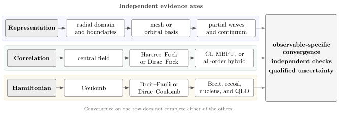
Atomic calculations mature along three partly independent axes. Moving to a larger CI or an all-order treatment does not repair an incomplete radial representation or a deficient Hamiltonian. Each axis needs its own convergence or comparison evidence, and the requested observable couples to them with different sensitivity.

A useful computational record treats the axes as separate coordinates:

$$\mathcal C = \left( \mathcal R_{\mathrm{1e}}, \mathcal C_{\mathrm{corr}}, \mathcal H_{\mathrm{phys}} \right),$$

where $\mathcal R_{\mathrm{1e}}$ identifies the radial/angular representation, $\mathcal C_{\mathrm{corr}}$ identifies the many-electron truncation, and $\mathcal H_{\mathrm{phys}}$ identifies the Hamiltonian and nuclear model. Quoting only “large basis” or “high-level method” does not locate a result in this space.

From Wavefunctions to Observables

The computational target is usually an observable, not a wavefunction norm or total energy. Each observable emphasizes different regions and components of the state.

Observable	Dominant sensitivities
binding or ionization energy	balanced correlation between charge states, orbital relaxation, relativistic terms
fine-structure interval	spin-dependent relativity, configuration mixing, Breit interaction
electric-dipole amplitude	valence tails, state balance, core polarization, transition operator
static polarizability	low-lying opposite-parity states, continuum/tail completeness, energy denominators
hyperfine constant	near-nuclear spin density, relativistic contraction, core polarization, nuclear moments
isotope shift	recoil operator, field shift, correlated density at the nucleus, nuclear radii
lifetime	all significant decay channels, transition frequencies, multipole amplitudes

Transition rates

For an electric-dipole transition from $i$ to $f$, a reduced-matrix-element form of the spontaneous rate is

$$A_{i\to f}^{E1} = \frac{\omega_{if}^3}{ 3\pi\epsilon_0\hbar c^3 } \frac{ |\langle\gamma_fJ_f\Vert\mathbf d\Vert \gamma_iJ_i\rangle|^2 }{ 2J_i+1 }.$$

Thus an amplitude error and a transition-frequency error enter differently; the rate scales as $\omega^3$. A common hybrid calculation uses a theoretical matrix element with an accurately measured transition frequency. That can be appropriate, but it must be labeled as a semiempirical prediction rather than a fully ab initio one.

The Transition Rates page owns radiative-rate conventions and selection rules.

Length and velocity forms

For exact eigenstates of a compatible nonrelativistic local Hamiltonian, commutator identities relate length- and velocity-form electric-dipole amplitudes. Schematically,

$$\langle f|\mathbf p|i\rangle = i(E_f-E_i) \langle f|\mathbf r|i\rangle.$$

Disagreement between the forms can expose incomplete wavefunctions or an inconsistent operator. Agreement is not proof of correctness: both forms can share missing correlation, and nonlocal potentials or relativistic Hamiltonians modify the simple identity. Gauge-form comparison is a diagnostic whose theoretical conditions must be stated.

Polarizabilities and tail completeness

For a nondegenerate state of total angular momentum $J_0$, a representative scalar dynamic polarizability in atomic units is

$$\alpha_0(\omega) = \frac{2}{3(2J_0+1)} \sum_n \frac{ (E_n-E_0) |\langle n\Vert D\Vert0\rangle|^2 }{ (E_n-E_0)^2-\omega^2 }.$$

The sum contains discrete and continuum states. In practice it is often partitioned into:

$$\alpha = \alpha_{\mathrm{main}} +\alpha_{\mathrm{tail}} +\alpha_{\mathrm{core}} +\alpha_{\mathrm{vc}},$$

where the last term corrects overlap or exclusion between core and valence descriptions. The low-lying “main” terms may use high-accuracy experimental energies and calculated matrix elements, while tails use a less expensive method. Every part needs an uncertainty estimate.

Finite-field extraction

An observable can sometimes be obtained as an energy derivative. In a static electric field $F$,

$$E(F) = E(0)-\mu F-\frac{1}{2}\alpha F^2+O(F^3).$$

A central difference gives

$$\alpha(F) \approx -\frac{E(F)-2E(0)+E(-F)}{F^2}.$$

Choose $F$ small enough for the quadratic regime but large enough that the energy difference exceeds solver noise. Vary the field and fit order. Finite-field and response-theory agreement is a valuable independent check only when both use comparably converged wavefunctions.

Sum rules and closure

For a complete set of exact nonrelativistic states, oscillator strengths obey the Thomas–Reiche–Kuhn sum rule. In one common convention for $N$ electrons,

$$\sum_n f_{0n}=N.$$

A finite pseudostate basis can approach this sum and thereby test broad dipole-space completeness. Satisfying one global sum rule does not guarantee accurate individual transitions, but severe failure identifies missing strength or an inconsistent operator.

State Tracking and Spectroscopic Identification

Levels of the same exact symmetry avoid crossing under a generic one-parameter variation and can exchange dominant configuration character. Energy ordering therefore becomes fragile precisely where atomic structure is most interesting.

Suppose $|\Psi_a(\lambda)\rangle$ are eigenstates as a basis, correlation model, or nuclear charge is varied. Track a state with an overlap matrix

$$O_{ab} = |\langle \Psi_a(\lambda) | \Psi_b(\lambda+\Delta\lambda) \rangle|^2.$$

When orbital sets differ, transform states to a common biorthogonal representation or compare invariant diagnostics. Useful identifiers include:

• exact $J$ and parity;
• dominant CSF weights;
• expectation values of $\mathbf L^2$ and $\mathbf S^2$ when meaningful;
• Landé $g$ factors;
• transition patterns;
• radial expectation values;
• and overlaps along the convergence sequence.

At a strong avoided crossing, a physical label may follow either adiabatic continuity or diabatic configuration character. State which convention is used. A table that silently swaps roots can imitate erratic numerical convergence.

Benchmark Ladder

A benchmark should isolate a claim. No single atom tests every part of a code or method, so build a ladder from analytic unit tests to realistic comparisons.

Hydrogenic unit tests

For a point nucleus of infinite mass, the nonrelativistic Coulomb energies are

$$E_n^{\mathrm{NR}} = -\frac{Z^2}{2n^2}.$$

A radial solver should reproduce:

• the spectrum and degeneracies permitted by the chosen Hamiltonian;
• radial node counts;
• analytic expectation values;
• orthonormality;
• the Coulomb virial theorem;
• and known dipole matrix elements or oscillator strengths.

For a point-nucleus Dirac equation, the binding energy is

$$\begin{aligned} \varepsilon_{n\kappa} ={}& c^2 \left[ 1+ \frac{(Z\alpha)^2}{ \left( n-|\kappa| +\sqrt{\kappa^2-(Z\alpha)^2} \right)^2 } \right]^{-1/2} -c^2. \end{aligned}$$

This tests $\kappa$ conventions, large/small-component coupling, kinetic balance, and the rest-energy convention. It does not test electron correlation.

Helium and few-electron ions

The nonrelativistic infinite-nuclear-mass helium ground-state energy is approximately

$$E_0(\mathrm{He}) = -2.903\,724\,377\,034\ E_h.$$

High-precision few-electron calculations provide many more digits, but the displayed value is already stringent enough for most implementation tests. It benchmarks:

• two-electron Coulomb integrals;
• singlet antisymmetry;
• electron correlation;
• cusp-sensitive basis convergence;
• and variational or partial-wave extrapolation.

It does not equal a directly measured total energy. Finite nuclear mass, relativity, QED, and the definition of the experimental reference must be added before theory–experiment comparison.

Helium-like ions across $Z$ are especially informative. At low $Z$, correlation is a substantial fraction of the binding correction; at higher $Z$, relativistic and nuclear effects grow. One isoelectronic sequence can therefore expose incorrect scaling or double counting.

Closed-shell and alkali-like tests

Closed-shell noble-gas-like systems test self-consistent fields, core correlation, and ionization energies. Alkali-like systems test a different architecture: one valence electron coupled to a polarizable closed core. Useful targets include:

• valence removal energies;
• fine-structure intervals;
• electric-dipole matrix elements;
• static scalar polarizabilities;
• and ground-state hyperfine constants.

No one observable certifies the others. Removal energies can be improved by a self-energy correction while an inconsistent effective dipole operator leaves transition amplitudes biased.

Multivalent and near-degenerate tests

Beryllium-like, alkaline-earth-like, and transition-metal-like systems test model-space design and configuration mixing. Choose levels with:

• clear single-configuration character;
• known avoided crossings or strong mixing;
• both parities;
• several $J$ sectors;
• and observables sensitive to different radial regions.

This prevents a benchmark set from rewarding a method only in its easiest regime.

Highly charged ions

Highly charged ions amplify relativistic and QED effects while often suppressing relative correlation through stronger nuclear binding. They test:

• Dirac spectra;
• Breit contributions;
• finite-nuclear-size sensitivity;
• radiative corrections;
• and the transition between LS-like and jj-like coupling.

At level crossings, correlation can again become nonperturbative despite large $Z$. Scaling arguments are guides, not substitutes for state analysis.

Experimental databases

Curated experimental data are indispensable for validation, but a database entry is not automatically a direct measurement with a transparent covariance matrix. Values may be optimized from networks of transitions, combined across experiments, or assigned an uncertainty from expert evaluation.

When using the NIST Atomic Spectra Database or another compilation, record:

• database release or access date;
• element, ion, isotope, and level identifiers;
• whether the value is observed, Ritz-optimized, or theoretical;
• units and conversion constants;
• uncertainty and any quality flag;
• and the original literature when the comparison is central.

Do not tune a model to a tabulated level and then count that same level as independent validation.

A compact benchmark matrix

Benchmark	Representation	Correlation	Hamiltonian	Observable/operator
hydrogenic bound states	radial boundary and basis	not tested	Coulomb or Dirac	energy and analytic moments
helium ground state	cusp and partial waves	two-electron correlation	nonrelativistic Coulomb	total energy
alkali removal energies	diffuse valence and core	core–valence all-order effects	relativistic mean field	energy differences
alkali E1 amplitudes	valence tails	core polarization	relativistic	effective dipole operator
heavy-ion fine structure	relativistic basis	residual correlation	Breit and QED sensitivity	intervals
isotope shifts	nuclear-region resolution	mass-polarization correlation	recoil and finite size	isotope-shift operators

The empty implication is deliberate: success in one column does not certify the others.

Verification Before Validation

Verification asks whether the implementation solves the stated equations. Validation asks whether those equations and approximations describe the physical target to the claimed accuracy. They require different evidence.

Algebraic and numerical verification

For an eigenpair, evaluate a residual

$$r_\nu = \|H\Psi_\nu-E_\nu\Psi_\nu\|.$$

In a generalized finite-basis problem,

$$\mathbf r_\nu = \mathbf H\mathbf c_\nu -E_\nu\mathbf S\mathbf c_\nu.$$

The residual must be interpreted relative to matrix norms, units, and conditioning. A tiny residual establishes an accurate eigenpair of the finite matrix. It says nothing about basis completeness or Hamiltonian adequacy.

For a normalized approximate state, the energy variance

$$\sigma_H^2 = \langle H^2\rangle-\langle H\rangle^2$$

vanishes for an exact eigenstate of the represented Hamiltonian. In variational and Monte Carlo contexts it is a useful state-quality diagnostic, but a small variance within an incomplete ansatz does not provide a universal error bound without spectral information.

Additional implementation checks include:

• Hermiticity to the expected floating-point tolerance;
• orthonormality or generalized orthonormality;
• exact zero matrix elements from parity and angular selection rules;
• determinant/CSF phase consistency;
• permutation symmetry;
• known one- and two-electron integral identities;
• and agreement between dense and sparse solvers on small matrices.

Convergence verification

Vary one truncation at a time while holding the others fixed:

$$Q(N_r,\ell_{\max},R_{\max},M_{\mathrm{CI}},k_{\mathrm{MBPT}},\ldots).$$

A practical sequence might be:

1. refine the radial grid or basis at fixed $\ell_{\max}$;
2. enlarge the cavity;
3. increase the maximum partial wave;
4. enlarge the reference and active configuration spaces;
5. raise perturbative order or excitation rank;
6. refine integral and iterative-solver tolerances;
7. repeat for the actual observable, not only the energy.

Simultaneously changing all cutoffs can hide cancellation and prevents a credible attribution of error.

Physical validation

Validation can use:

• analytic limits;
• independent implementations;
• calculations organized by a different method;
• isoelectronic and scaling trends;
• redundant observable forms;
• sum rules;
• and measurements not used for calibration.

Agreement with one experiment is weakest when adjustable parameters were chosen after seeing it. Predicting several observables with different sensitivity, using parameters fixed elsewhere, is stronger evidence.

Convergence and Uncertainty Ledger

An atomic result should carry an error ledger matched to the observable. A useful decomposition is

$$\delta Q \leftarrow \left\{ \delta_{\mathrm{repr}}, \delta_{\mathrm{corr}}, \delta_{\mathrm{Ham}}, \delta_{\mathrm{op}}, \delta_{\mathrm{num}}, \delta_{\mathrm{data}} \right\}.$$

The arrow is intentional: these components need not be statistically independent and should not automatically be added in quadrature.

Component	Evidence that can constrain it
representation	nested radial bases, boxes, meshes, and partial-wave extrapolations
correlation	active-space increments, perturbative order, triples estimates, independent many-body methods
Hamiltonian	Breit, recoil, finite-size, and QED increments; alternative nuclear models
operator	effective-operator order, length/velocity comparison, finite-field/response comparison
numerical	eigensolver residuals, integral thresholds, precision, conditioning
external data	constants, nuclear radii and moments, empirical energies, experimental covariance

Differences are not automatically uncertainties

The difference between two approximations is evidence, not a probability distribution. For example:

• a basis increment estimates omitted basis contributions only if the sequence is in a stable convergence regime;
• a triples correction can proxy higher excitations but may miss multireference failure;
• length–velocity disagreement can diagnose wavefunction imbalance but is not a calibrated confidence interval;
• method spread can underestimate shared systematic bias.

A defensible uncertainty argument explains why each proxy should bound or represent the omitted effects and tests that explanation on benchmarks.

Correlated cancellations

Transition energies are differences,

$$\Delta E=E_b-E_a.$$

Large common errors can cancel. This is beneficial but creates correlation between uncertainties. Computing $E_a$ and $E_b$ with unrelated orbital spaces may lose the cancellation, whereas a state-averaged calculation can improve balance at the cost of each individual state’s variational optimum.

Report both absolute contributions and their effect on the interval when possible. Do not combine uncertainties for $E_a$ and $E_b$ as if they were independent unless that assumption is justified.

Significant digits

Print enough guard digits to reproduce derived quantities, but distinguish them from claimed accuracy. A result such as

$$Q=12.347\,81(24)$$

states an uncertainty of $0.000\,24$ in the same units. A long decimal without an uncertainty is not a precision claim; it is merely solver output.

Reproducibility Record

A mature atomic-structure result should preserve:

• the Hamiltonian and every correction included;
• the nuclear charge, mass, radius, moments, and source data;
• orbital conventions and reference potential;
• radial domain, mapping, basis family, and angular cutoffs;
• CSF generation rules and resulting dimensions by symmetry;
• frozen-core and active-space definitions;
• solver, integral, and selection thresholds;
• state-identification diagnostics;
• operator dressing and any experimental substitutions;
• convergence tables and uncertainty construction;
• software version, environment, random seeds if applicable;
• and machine-readable output with units and provenance.

A source archive without the generated configuration list or numerical input is often insufficient. Conversely, a configuration list without code version and operator conventions cannot reproduce a precision result. The Software, Notebooks, and Benchmarks registry owns the general artifact policy.

Method-Selection Workflow

The following workflow keeps the physical and numerical decisions in the right order.

Step 1: Define the target and tolerance

Specify the isotope, charge state, symmetry, state-identification rule, observable, units, and desired uncertainty.

Step 2: Choose the Hamiltonian

Estimate the sizes of correlation, relativistic, recoil, finite-size, Breit, and QED effects. Select a nonrelativistic or relativistic starting point that does not force a large physical effect into an uncontrolled correction.

Step 3: Diagnose state structure

Use central-field or mean-field orbitals to inspect configurations and energy separations. If several configurations of the same symmetry are close, put them in a model or reference space from the beginning.

Step 4: Design the one-electron representation

Resolve the nucleus, core, valence, diffuse tail, and continuum according to the observable. Choose radial and angular convergence sequences before running the largest calculation.

Step 5: Select the correlation organization

Use CI or multiconfiguration methods for transparent strong mixing, MBPT or all-order methods for a well-separated reference, and hybrid effective Hamiltonians when a few valence electrons interact above a correlated core.

Step 6: Construct observables consistently

Use effective operators or response equations at a level balanced with the Hamiltonian. Track all channels, continuum tails, and experimental substitutions.

Step 7: Verify each axis

Run analytic unit tests, residual checks, radial/angular convergence, configuration or order convergence, and state tracking.

Step 8: Validate and budget uncertainty

Compare independent methods and measurements not used in calibration. Build an observable-specific uncertainty ledger and round the result accordingly.

Common Failure Modes

Converging the solver instead of the physics

An SCF threshold of $10^{-12}$ or an eigensolver residual of $10^{-14}$ describes the finite numerical problem. It does not imply twelve or fourteen correct digits in the continuum, correlated, physical atom.

Calling every basis function an orbital

Primitive radial or Gaussian functions span a one-electron space. Physical interpretation usually belongs to optimized linear combinations, natural orbitals, or Dyson orbitals. Confusing primitives with states obscures invariance under basis rotations.

Comparing unequal Hamiltonians

Two energies cannot isolate a correlation method if one uses a finite nucleus and Breit interaction while the other uses a point-nucleus Coulomb model. Align the Hamiltonians before attributing a difference.

Double counting fitted physics

A model potential fitted to experimental levels may already absorb correlation and relativistic effects. Adding explicit corrections calibrated to the same levels can count them twice.

Treating orbital energies as a spectrum

Hartree–Fock or Kohn–Sham orbital differences are not generally neutral excitation energies. Compute the appropriate many-electron energy difference or response quantity.

Ignoring root flipping

Energy-sorted level indices can swap at avoided crossings or as a CI space changes. Track overlaps and observables, then document the labeling convention.

Optimizing only the total energy

The energy is stationary with respect to first-order wavefunction errors; many other observables are not. Validate the requested matrix element, density, or derivative directly.

Using gauge agreement as certification

Length and velocity forms can agree because they share an approximation. Treat agreement as one diagnostic among several, not an accuracy theorem for a truncated calculation.

Hiding empirical substitutions

Replacing theoretical level splittings by measured values can substantially improve rates or polarizabilities. It also changes the provenance of the result. Label the substitution and propagate experimental uncertainty.

Extrapolating before reaching an asymptotic regime

Two or three smooth-looking points do not establish the theoretical power law behind a basis or partial-wave tail. Vary fit windows and compare plausible forms.

Reporting a universal method uncertainty

One percentage does not apply equally to energies, E1 amplitudes, hyperfine constants, and isotope shifts. Uncertainty belongs to a defined observable in a defined state.

Exercises

Exercise 1: Reference-potential cancellation

Starting from

$$H = \sum_i(h_i+U_i) + \left( V_{ee}-\sum_iU_i \right),$$

show that the exact Hamiltonian is independent of $U$. Explain why a finite-order perturbation result can still depend on the chosen potential.

Solution

The two appearances of $U$ cancel algebraically:

$$\sum_i(h_i+U_i) +V_{ee}-\sum_iU_i = \sum_i h_i+V_{ee}.$$

Therefore exact eigenvalues and observables cannot depend on the partition. Perturbation theory, however, treats $\sum_i(h_i+U_i)$ exactly and truncates the expansion in $V_{ee}-\sum_iU_i$. Changing $U$ moves contributions between orders. Terms needed to restore partition independence may lie beyond the truncation. The residual $U$ dependence is consequently a diagnostic of omitted orders, provided all subtraction terms at the retained order were included.

Exercise 2: Radial boundary conditions

For a Coulomb potential, insert $u(r)\sim r^s$ into the radial Schrödinger equation and determine the regular exponent near $r=0$. Why is the other solution rejected?

Solution

Near the origin, the centrifugal term is more singular than $-Z/r$ for $\ell>0$. Keeping the $r^{s-2}$ terms gives

$$-\frac12s(s-1)r^{s-2} +\frac{\ell(\ell+1)}{2}r^{s-2} =0.$$

Thus

$$s(s-1)=\ell(\ell+1),$$

with roots $s=\ell+1$ and $s=-\ell$. The first gives $u\propto r^{\ell+1}$ and $\psi=uY_{\ell m}/r\propto r^\ell$, which is regular. The second gives $\psi\propto r^{-\ell-1}$ and is not square integrable for $\ell\ge1$; for $\ell=0$ it is singular and incompatible with the physical self-adjoint boundary condition. Therefore the regular numerical solution uses $s=\ell+1$.

Exercise 3: Variational monotonicity

Let $\mathcal V_M\subset\mathcal V_{M+1}$ be nested CI spaces of the same symmetry. Prove that their lowest eigenvalues satisfy $E_0^{(M+1)}\le E_0^{(M)}$. Give two reasons this fact may appear violated in a production calculation.

Solution

The Rayleigh–Ritz characterization is

$$E_0^{(M)} = \min_{\substack{\psi\in\mathcal V_M\\\|\psi\|=1}} \langle\psi|H|\psi\rangle.$$

Every normalized vector in $\mathcal V_M$ also belongs to $\mathcal V_{M+1}$. Minimizing over the larger set cannot give a larger value:

$$E_0^{(M+1)} \le E_0^{(M)}.$$

An apparent violation can occur if the orbital sets were reoptimized so that the finite spaces are not nested, if different roots or symmetries were compared, if a nonvariational perturbative correction was added, or if numerical errors exceed the energy increment.

Exercise 4: Energy convergence versus SCF convergence

Near a stationary Hartree–Fock solution, an orbital rotation is parameterized by a small amplitude $\kappa$. Explain why the energy error can be $O(\kappa^2)$ while the orbital-gradient residual is $O(\kappa)$. What does this imply for stopping criteria?

Solution

At a stationary point, the first variation of the energy vanishes:

$$E(\kappa) = E(0) +\frac12 \kappa^{\mathsf T}\mathbf H_{\mathrm{orb}}\kappa +O(\kappa^3).$$

The gradient is

$$\nabla_\kappa E = \mathbf H_{\mathrm{orb}}\kappa +O(\kappa^2).$$

Thus successive energies can look converged quadratically while the orbitals remain wrong to first order. A robust SCF stopping rule checks an orbital-gradient or commutator residual as well as energy and density changes.

Exercise 5: A small denominator

Consider a two-state Hamiltonian

$$H= \begin{pmatrix} 0 & 0.02\\ 0.02 & 0.01 \end{pmatrix}$$

in hartree. Treat the off-diagonal coupling perturbatively about the first state, then compare the second-order energy with the exact lower eigenvalue. What method change is indicated?

Solution

The second-order correction to the first diagonal state is

$$E^{(2)} = \frac{0.02^2}{0-0.01} =-0.04\ E_h.$$

The exact eigenvalues are

$$E_\pm = \frac{0.01\pm \sqrt{0.01^2+4(0.02)^2}}{2},$$

so

$$E_-\approx-0.0156\ E_h.$$

The perturbative correction is larger in magnitude than the level separation and badly overshoots the exact shift. Both configurations should be included in a model space and diagonalized together; residual coupling to more distant states can then be treated perturbatively.

Exercise 6: Nonrelativistic limit of the Dirac benchmark

For the hydrogenic Dirac expression, define

$$\gamma=\sqrt{\kappa^2-(Z\alpha)^2}.$$

Show at leading order in $Z\alpha$ that the binding energy is $-Z^2/(2n^2)$ hartree.

Solution

For small $Z\alpha$,

$$\gamma = |\kappa| -\frac{(Z\alpha)^2}{2|\kappa|} +O((Z\alpha)^4).$$

Therefore the denominator $n-|\kappa|+\gamma=n+O((Z\alpha)^2)$. To leading order,

$$\begin{aligned} \varepsilon_{n\kappa} &= c^2 \left[ 1+\frac{(Z\alpha)^2}{n^2} \right]^{-1/2} -c^2 \\ &= -\frac{c^2(Z\alpha)^2}{2n^2} +O((Z\alpha)^4c^2). \end{aligned}$$

Since $c=1/\alpha$ in atomic units,

$$\varepsilon_{n\kappa} = -\frac{Z^2}{2n^2} +O(Z^4\alpha^2).$$

The leading term is independent of $\kappa$, recovering the nonrelativistic Coulomb degeneracy.

Exercise 7: Observable-specific validation

Design separate validation plans for (a) an alkali ionization energy, (b) an E1 transition amplitude, and (c) a hyperfine constant. Name one representation, correlation, Hamiltonian, and operator check for each.

Solution

A defensible plan could include:

Target	Representation	Correlation	Hamiltonian	Operator or comparison
ionization energy	diffuse valence and cavity convergence	core–valence order or triples increments	Dirac–Coulomb plus Breit/QED increments	balanced neutral/ion energy difference; compare measured threshold
E1 amplitude	valence-tail and pseudostate completeness	core-polarization and valence-correlation increments	relativistic orbitals where needed	length/velocity forms and finite-field or lifetime comparison
hyperfine constant	dense near-nuclear mesh and finite nucleus	core polarization and spin polarization	finite-size, Breit, and radiative sensitivity	dressed hyperfine operator and stated nuclear moment

The plans differ because each observable weights the wavefunction differently. An energy-only benchmark is not enough for either matrix element.

Exercise 8: Building an uncertainty ledger

A polarizability calculation changes by $0.18$ a.u. under the final basis extension, by $0.31$ a.u. when estimated triples are added, and by $0.07$ a.u. when Breit and QED corrections are included. Length and velocity forms differ by $0.12$ a.u. Explain why

$$\sqrt{0.18^2+0.31^2+0.07^2+0.12^2}$$

is not automatically a justified uncertainty.

Solution

The four numbers are changes or discrepancies, not necessarily independent random standard deviations. The basis increment may share correlation error with the triples increment. The length–velocity difference can respond to both basis and correlation incompleteness, so adding it again may double count. The Breit/QED value is a correction, not the uncertainty of that correction.

A defensible ledger would first assign meanings: extrapolate the basis sequence, estimate omitted excitations using benchmarks or multiple approximations, attach an uncertainty to the relativistic correction, and use gauge disagreement as a diagnostic constraint. Correlations among those estimates should then determine whether to combine them linearly, in quadrature, through a covariance model, or by a conservative envelope.

Exercise 9: Tracking a mixed pair

Two computed levels of the same $J^\pi$ have dominant configuration weights $(0.80,0.15)$ at one active-space size and $(0.35,0.60)$ at the next. Their energy order is unchanged. What additional data would you use to decide whether the states exchanged character?

Solution

Compute overlaps between old and new eigenvectors after expressing them in a common orbital representation. Also compare Landé $g$ factors, transition patterns, radial expectation values, and the full set of leading CSF weights. If the largest overlap connects the old lower root to the new upper root, the diabatic configuration labels exchanged even though the energy order did not. If each energy-ordered root has the largest self-overlap while its configuration weights rotate smoothly, the states are following adiabatic branches through strong mixing. The published labels should state which continuity convention is used.

Key Takeaways

• Atomic-structure quality has at least three independent axes: one-electron representation, electron correlation, and Hamiltonian fidelity.
• Central fields and Hartree–Fock supply useful reference orbitals, not exact spectra.
• CI treats strong configuration mixing transparently; MBPT and all-order methods are efficient when the reference and model space are well chosen.
• Relativistic calculations require more than replacing Schrödinger orbitals by Dirac spinors: kinetic balance, positive-energy projection, nuclear models, Breit terms, and QED provenance matter.
• Validate the requested observable. Energies, transition amplitudes, polarizabilities, and hyperfine constants probe different errors.
• Hydrogenic, helium, isoelectronic, multivalent, and heavy-ion tests occupy different rungs of a benchmark ladder.
• Solver residuals verify a finite calculation; convergence studies and independent comparisons support physical claims.
• Uncertainty increments are not automatically independent standard deviations.

Cross-Links

• Computational AMO and Quantum Chemistry
• Electronic Structure Methods Map
• Radial Schrödinger Equation
• Boundary Conditions for Radial Wavefunctions
• Central-Field Approximation
• Hartree Method
• Hartree–Fock for Atoms
• Hartree–Fock Notebook
• Atomic Correlation Methods Overview
• Helium Atom
• Fine Structure
• Hyperfine Structure
• Sparse Eigensolvers
• Error Estimates
• Computational QM Roadmap
• Computational QM References

References

1. C. Froese Fischer, T. Brage, and P. Jönsson, Computational Atomic Structure: An MCHF Approach, Institute of Physics Publishing (1997).
2. W. R. Johnson, Atomic Structure Theory: Lectures on Atomic Physics, Springer (2007), doi:10.1007/978-3-540-68013-0.
3. I. P. Grant, Relativistic Quantum Theory of Atoms and Molecules: Theory and Computation, Springer (2007), doi:10.1007/978-0-387-35069-1.
4. I. Lindgren and J. Morrison, Atomic Many-Body Theory, 2nd ed., Springer (1986), doi:10.1007/978-3-642-61640-2.
5. I. Lindgren, Relativistic Many-Body Theory: A New Field-Theoretical Approach, Springer (2011), doi:10.1007/978-1-4419-8309-1.
6. M. S. Safronova and W. R. Johnson, “All-Order Methods for Relativistic Atomic Structure Calculations,” Advances in Atomic, Molecular and Optical Physics 55, 191–233 (2008), doi:10.1016/S1049-250X(07)55004-4.
7. H. Bachau, E. Cormier, P. Decleva, J. E. Hansen, and F. Martín, “Applications of B-splines in Atomic and Molecular Physics,” Reports on Progress in Physics 64, 1815–1943 (2001), doi:10.1088/0034-4885/64/12/205.
8. C. Froese Fischer, G. Tachiev, G. Gaigalas, and M. R. Godefroid, “An MCHF Atomic-Structure Package for Large-Scale Calculations,” Computer Physics Communications 176, 559–579 (2007), doi:10.1016/j.cpc.2007.01.006.
9. P. Jönsson, G. Gaigalas, J. Bieroń, C. Froese Fischer, and I. P. Grant, “New Version: Grasp2K Relativistic Atomic Structure Package,” Computer Physics Communications 184, 2197–2203 (2013), doi:10.1016/j.cpc.2013.02.016.
10. W. R. Johnson, S. A. Blundell, and J. Sapirstein, “Finite Basis Sets for the Dirac Equation Constructed from B Splines,” Physical Review A 37, 307–315 (1988), doi:10.1103/PhysRevA.37.307.
11. V. A. Dzuba, V. V. Flambaum, and M. G. Kozlov, “Combination of the Many-Body Perturbation Theory with the Configuration-Interaction Method,” Physical Review A 54, 3948–3959 (1996), doi:10.1103/PhysRevA.54.3948.
12. S. A. Blundell, W. R. Johnson, and J. Sapirstein, “Relativistic All-Order Calculations of Energies and Matrix Elements in Cesium,” Physical Review A 43, 3407–3418 (1991), doi:10.1103/PhysRevA.43.3407.
13. M. S. Safronova, M. G. Kozlov, W. R. Johnson, and D. Jiang, “Development of a Configuration-Interaction Plus All-Order Method for Atomic Calculations,” Physical Review A 80, 012516 (2009), doi:10.1103/PhysRevA.80.012516.
14. M. F. Gu, “The Flexible Atomic Code,” Canadian Journal of Physics 86, 675–689 (2008), doi:10.1139/P07-197.
15. T. Kato, “On the Eigenfunctions of Many-Particle Systems in Quantum Mechanics,” Communications on Pure and Applied Mathematics 10, 151–177 (1957), doi:10.1002/cpa.3160100201.
16. G. W. F. Drake, ed., Springer Handbook of Atomic, Molecular, and Optical Physics, Springer (2006), doi:10.1007/978-0-387-26308-3.
17. A. Kramida, Yu. Ralchenko, J. Reader, and the NIST ASD Team, NIST Atomic Spectra Database, National Institute of Standards and Technology, doi:10.18434/T4W30F, accessed 2026-07-26.
18. J. S. Sims and S. A. Hagstrom, “Hylleraas-Configuration-Interaction Study of the $1\,{}^1S$ Ground State of Neutral Helium,” Physical Review A 83, 032518 (2011), doi:10.1103/PhysRevA.83.032518.

Further Study

For boundary-value methods, implement the hydrogenic problem with Radial Schrödinger Solvers. For a nonlinear orbital problem, continue to the Hartree–Fock Notebook, which carries the same convergence and validation discipline into a self-consistent field.