Hartree–Fock Notebook

This notebook solves a genuine self-consistent-field problem without hiding the integral engine or the convergence tests. Two opposite-spin electrons occupy one spatial orbital expanded in normalized, one-centre $s$-type Gaussian functions. Every overlap, kinetic, nuclear-attraction, and electron-repulsion integral is analytic. The only external dependency is NumPy.

For the published eight-function basis, the retained program obtains

$$E_{\mathrm{RHF}}^{(8)} = -2.861\,492\,180\,485\,973E_{\mathrm h}$$

after 16 undamped fixed-point iterations. The final density has electron count

$$\operatorname{Tr}(PS) = 1.999\,999\,999\,999\,994,$$

and the generalized Fock residual is approximately $1.14\times10^{-13}$. Yet the energy remains

$$1.878\,151\,262\,660\times10^{-4}E_{\mathrm h}$$

above a high-precision Hartree–Fock-limit reference. Algebraic convergence of the self-consistency loop is therefore not the same claim as convergence of the one-electron basis.

Run the investigation. The program and retained results below support the stated experiment. Follow Running an Experiment for environment and output-directory guidance. The recorded evidence applies to its stated parameters and environment.

Canonical Scope

Hartree–Fock Approximation owns the determinant variational derivation, direct and exchange operators, spin variants, occupied-projector formulation, stability questions, and general Roothaan–Hall equations. Hartree–Fock for Atoms owns the atomic specialization, radial equations, closed and open shells, atomic exchange, asymptotic behavior, and interpretation of atomic orbitals. Helium Atom owns the physical helium spectrum and precision hierarchy.

This page owns the reproducible computational experiment:

• construct all matrix elements from declared Gaussian exponents;
• solve a nonorthogonal generalized eigenproblem;
• build a closed-shell density and its Fock matrix;
• iterate them to self-consistency without an accelerator;
• expose a complete two-function matrix example;
• separate SCF, basis, and method errors;
• validate density, integral, eigenpair, and energy identities;
• compare with retained Hartree–Fock and correlated references;
• and state what an occupied orbital energy does and does not mean.

The implementation is intentionally small enough to audit line by line. It is not a production quantum-chemistry package, a general molecular integral engine, or a benchmark for advanced SCF accelerators.

Reproducibility Contract

Item	Notebook choice
system	neutral helium, nuclear charge $Z=2$, two electrons
Hamiltonian	nonrelativistic Coulomb Hamiltonian, infinite-mass point nucleus
state	closed-shell $1s^2\,{}^1S$ ground-state model
ansatz	one doubly occupied spatial orbital, restricted Hartree–Fock
representation	nested uncontracted one-centre normalized $s$ Gaussians
integrals	analytic overlap, kinetic, nuclear-attraction, and two-electron integrals
eigensolver	symmetric orthogonalization followed by a Hermitian eigensolve
SCF map	undamped density fixed-point iteration from a core-Hamiltonian guess
stopping rule	density RMS below $10^{-12}$ and energy change below $10^{-13}E_{\mathrm h}$
arithmetic	IEEE 754 binary64 through NumPy
randomness	none
artifacts	Python program, two CSV files, two JSON files, SVG figure

The code reports more digits than the physical model justifies so that deterministic reruns and algebraic identities can be tested. Those digits must not be mistaken for accuracy relative to exact helium.

Physical Model

In Hartree atomic units,

$$\hbar=m_e=e=4\pi\epsilon_0=1.$$

The clamped-nucleus electronic Hamiltonian is

$$H = \sum_{i=1}^{2} \left( -\frac12\nabla_i^2-\frac{Z}{r_i} \right) +\frac{1}{r_{12}}, \qquad Z=2.$$

There is no nuclear-repulsion constant because this is a one-nucleus atom. The energy zero is a bare nucleus and two electrons at rest at infinite separation.

Restricted closed-shell state

The normalized spatial orbital $\phi(\mathbf r)$ is occupied by one $\alpha$-spin electron and one $\beta$-spin electron. The determinant may be written

$$\Phi(x_1,x_2) = \frac{1}{\sqrt2} \begin{vmatrix} \phi(\mathbf r_1)\alpha(1) & \phi(\mathbf r_1)\beta(1) \\ \phi(\mathbf r_2)\alpha(2) & \phi(\mathbf r_2)\beta(2) \end{vmatrix}.$$

Equivalently, its spatial part is the symmetric product $\phi(\mathbf r_1)\phi(\mathbf r_2)$ and its spin part is the singlet. The opposite-spin pair has no exchange integral between distinct spin-orbitals, but the closed-shell Fock expression still contains exchange bookkeeping. That bookkeeping cancels self-interaction and leaves one Coulomb field acting on either occupied electron.

For one normalized spatial orbital, define

$$h_\phi = \langle\phi|h|\phi\rangle, \qquad J_\phi = \iint \frac{ |\phi(\mathbf r_1)|^2 |\phi(\mathbf r_2)|^2 }{ r_{12} } \,d^3r_1\,d^3r_2,$$

where

$$h=-\frac12\nabla^2-\frac{Z}{r}.$$

Then

$$E_{\mathrm{RHF}} = 2h_\phi+J_\phi,$$

while the occupied canonical orbital satisfies

$$\epsilon_\phi = h_\phi+J_\phi.$$

These equations already warn that the total energy is not twice the orbital energy.

Why helium is a useful SCF demonstrator

Helium is simple but not trivial:

• there is only one occupied spatial orbital, so spin and occupation bookkeeping stay transparent;
• electron repulsion makes the optimal orbital depend on its own density;
• a finite nonorthogonal basis produces a genuine generalized eigenproblem;
• the SCF loop is nonlinear even though each diagonalization is linear;
• an accurate Hartree–Fock limit and a much more accurate correlated energy are available for comparison;
• and the distinction between orbital relaxation and electron correlation is unusually clean.

Helium does not test multiple occupied orbitals, same-spin exchange between different orbitals, near-degeneracy, symmetry breaking, open shells, or multiple SCF stationary points. Those omissions matter when generalizing the lessons.

Finite One-Electron Basis

The spatial orbital is expanded as

$$\phi(\mathbf r) = \sum_{\mu=1}^{K}C_\mu\chi_\mu(\mathbf r).$$

Each basis function is a normalized primitive Gaussian centred on the nucleus:

$$\chi_\mu(\mathbf r) = N_\mu e^{-\alpha_\mu r^2}, \qquad N_\mu = \left( \frac{2\alpha_\mu}{\pi} \right)^{3/4}, \qquad \alpha_\mu>0.$$

The exponent has dimensions $a_0^{-2}$ when dimensions are restored. A large $\alpha_\mu$ describes a tight function near the nucleus; a small exponent describes a diffuse function.

Published nested sequence

The complete retained set is the even-tempered sequence

$$\alpha_k=0.2\times3^k, \qquad k=0,\ldots,7,$$

but functions are inserted in the order

$$\left( 0.6,\, 1.8,\, 0.2,\, 5.4,\, 16.2,\, 48.6,\, 145.8,\, 437.4 \right).$$

This ordering starts with two valence-scale functions and then adds diffuse and successively tighter flexibility. Every $K$-function space is contained in the next one, so an exactly minimized variational energy cannot increase with $K$.

The ordering is pedagogical, not an optimized basis design. A production basis would normally use carefully optimized and often contracted functions, polarization functions for nonspherical environments, and diffuse functions selected for the target property.

Gaussian strengths and limitations

Products of Gaussians are analytically convenient. Even the four-index electron-repulsion integrals reduce here to a closed expression. A single Gaussian nevertheless has zero radial derivative at the nucleus:

$$\left. \frac{d}{dr} e^{-\alpha r^2} \right|_{r=0} = 0.$$

The exact Coulombic orbital has a nuclear cusp. A linear combination of finitely many centred $s$ Gaussians therefore cannot satisfy the cusp condition exactly. Tight functions imitate the cusp over a finite region but do not change the analytic behavior at $r=0$.

This is one reason a modest Gaussian expansion can give a good total energy while pointwise or contact properties converge more slowly.

Analytic Integral Engine

All basis functions share the same centre. Define

$$p_{\mu\nu} = \alpha_\mu+\alpha_\nu, \qquad q_{\lambda\sigma} = \alpha_\lambda+\alpha_\sigma.$$

The notebook uses chemists’ two-electron notation

$$(\mu\nu|\lambda\sigma) = \iint \chi_\mu(\mathbf r_1) \chi_\nu(\mathbf r_1) \frac{1}{r_{12}} \chi_\lambda(\mathbf r_2) \chi_\sigma(\mathbf r_2) \,d^3r_1\,d^3r_2.$$

All functions are real.

Overlap

The overlap matrix is

$$S_{\mu\nu} = \langle\chi_\mu|\chi_\nu\rangle = N_\mu N_\nu \left( \frac{\pi}{p_{\mu\nu}} \right)^{3/2}.$$

Individual primitives are normalized, so $S_{\mu\mu}=1$, but different primitives are not orthogonal.

Kinetic energy

For $s$ Gaussians at the same centre,

$$T_{\mu\nu} = \left\langle \chi_\mu \left| -\frac12\nabla^2 \right| \chi_\nu \right\rangle = S_{\mu\nu} \frac{ 3\alpha_\mu\alpha_\nu }{ p_{\mu\nu} }.$$

The matrix is symmetric, as required for a Hermitian one-electron operator.

Nuclear attraction

With a point nucleus at the common centre,

$$V_{\mu\nu} = \left\langle \chi_\mu \left| -\frac{Z}{r} \right| \chi_\nu \right\rangle = -Z N_\mu N_\nu \frac{2\pi}{p_{\mu\nu}}.$$

The core Hamiltonian matrix is

$$h_{\mu\nu} = T_{\mu\nu}+V_{\mu\nu}.$$

Electron repulsion

The four-index integral is

$$(\mu\nu|\lambda\sigma) = N_\mu N_\nu N_\lambda N_\sigma \frac{ 2\pi^{5/2} }{ p_{\mu\nu} q_{\lambda\sigma} \sqrt{ p_{\mu\nu}+q_{\lambda\sigma} } }.$$

The implementation constructs the full $K^4$ tensor because $K\leq8$. It checks the permutation symmetries

$$\begin{aligned} (\mu\nu|\lambda\sigma) &= (\nu\mu|\lambda\sigma),\\ &= (\mu\nu|\sigma\lambda),\\ &= (\lambda\sigma|\mu\nu). \end{aligned}$$

A production integral engine would exploit these symmetries, screen small integrals, and avoid materializing a dense tensor when the system is large.

The Nonorthogonal Eigenproblem

Normalization of the molecular-orbital coefficient vector is metric normalization:

$$\mathbf C^{\mathsf T}S\mathbf C=1.$$

Stationarity of the finite-basis Hartree–Fock energy gives the Roothaan equation

$$F\mathbf C = S\mathbf C\epsilon.$$

Solving $F\mathbf C=\mathbf C\epsilon$ would be wrong unless $S=I$. The primitive Gaussians here overlap strongly, so that mistake is numerically visible even in the two-function example.

Symmetric orthogonalization

Diagonalize the positive-definite overlap matrix:

$$S = U s U^{\mathsf T},$$

where $s$ is diagonal with positive eigenvalues. Define

$$X = S^{-1/2} = U s^{-1/2}U^{\mathsf T}.$$

Then

$$X^{\mathsf T}SX=I.$$

The generalized problem becomes the ordinary symmetric problem

$$\left( X^{\mathsf T}FX \right) \widetilde{\mathbf C} = \widetilde{\mathbf C}\epsilon,$$

and the original coefficients are recovered through

$$\mathbf C=X\widetilde{\mathbf C}.$$

The code symmetrizes the transformed Fock matrix before diagonalization to remove tiny floating-point antisymmetric components.

Conditioning

If two basis functions become nearly linearly dependent, the smallest overlap eigenvalue approaches zero and $S^{-1/2}$ amplifies roundoff. The notebook records

$$\kappa(S) = \frac{s_{\max}}{s_{\min}}.$$

For the final eight-function basis,

$$\kappa(S) = 280.949\,066\,266\,0856.$$

This is not severe in binary64 arithmetic, but it is large enough to make conditioning part of the evidence. The code refuses an overlap eigenvalue at or below $10^{-11}$ instead of silently dividing by it.

Density and Fock Construction

For one doubly occupied real spatial orbital, the closed-shell density matrix is

$$P_{\mu\nu} = 2C_\mu C_\nu.$$

The factor of two is the occupation. With the integral ordering defined above, the Fock matrix is

$$F_{\mu\nu} = h_{\mu\nu} + \sum_{\lambda\sigma} P_{\lambda\sigma} \left[ (\mu\nu|\lambda\sigma) -\frac12 (\mu\lambda|\nu\sigma) \right].$$

The first term in brackets is Coulomb and the second is closed-shell exchange. Index permutations that look harmless on paper can change the exchange contraction in code; the explicit convention is therefore part of the reproducibility contract.

Total electronic energy

Once $P$ and its self-consistent $F[P]$ are known,

$$E_{\mathrm{el}} = \frac12 \sum_{\mu\nu} P_{\mu\nu} \left( h_{\mu\nu}+F_{\mu\nu} \right).$$

The factor $1/2$ prevents double counting the two-electron field already present in each orbital equation. In matrix notation for real symmetric matrices,

$$E_{\mathrm{el}} = \frac12 \operatorname{Tr} \left[ P(h+F) \right].$$

There is no separate nuclear-repulsion term for helium.

Metric density identities

The nonorthogonal-basis density must satisfy

$$\operatorname{Tr}(PS)=2$$

and, for a rank-one closed-shell projector,

$$PSP=2P.$$

Checking $P^2=2P$ would incorrectly assume an orthonormal basis. The metric-aware identity is the appropriate idempotency test.

At self-consistency, the occupied subspace is invariant under its own Fock operator. A useful atomic-orbital residual is

$$R = FPS-SPF.$$

The notebook reports $\lVert R\rVert_{\mathrm F}$, the Frobenius norm. A small energy change alone does not guarantee a small orbital-gradient residual.

Self-Consistency Loop

The Fock matrix depends on the density, while the density is built from Fock eigenvectors:

$$P \longmapsto F[P] \longmapsto \mathbf C_{\mathrm{occ}}[F] \longmapsto P'.$$

A self-consistent density is a fixed point $P'=P$.

Initial guess

The program begins by solving the core-Hamiltonian problem

$$h\mathbf C^{(0)} = S\mathbf C^{(0)}\epsilon^{(0)}.$$

The lowest vector supplies $P^{(0)}$. This guess includes nuclear attraction and kinetic energy but no electron repulsion.

Iteration implemented

For $n=0,1,\ldots$:

1. Build $F[P^{(n)}]$.
2. Solve $F[P^{(n)}]\mathbf C=S\mathbf C\epsilon$.
3. Occupy the lowest spatial orbital and construct $P^{(n+1)}$.
4. Rebuild $F[P^{(n+1)}]$ for self-consistent energy and residual diagnostics.
5. Stop only when both density and energy criteria pass.

The density criterion is

$$\operatorname{RMS} \left( \Delta P \right) = \left[ \frac{1}{K^2} \sum_{\mu\nu} \left( P_{\mu\nu}^{(n+1)} -P_{\mu\nu}^{(n)} \right)^2 \right]^{1/2} < 10^{-12}.$$

The energy criterion is

$$\left| E^{(n+1)}-E^{(n)} \right| < 10^{-13}E_{\mathrm h}.$$

After convergence, the program performs one final Fock build and generalized eigensolve before reporting eigenpair diagnostics.

Why no damping or DIIS

The helium map converges smoothly from the core guess, so undamped fixed-point iteration exposes the raw nonlinear map. It is not a recommendation for general calculations. Larger systems can oscillate, converge slowly, or approach an unintended stationary point.

Density damping replaces the new density by

$$P_{\mathrm{mix}}^{(n+1)} = (1-\eta)P^{(n)} +\eta P_{\mathrm{out}}^{(n+1)}, \qquad 0<\eta\leq1.$$

Pulay’s direct inversion in the iterative subspace uses a history of residuals to extrapolate a better Fock matrix or density. Level shifting, occupation control, augmented-Hessian methods, and trust-region approaches address other failure modes. An accelerator changes the solver path, not the Hartree–Fock stationary equations.

Minimal Two-Function Example

The minimal demonstrator uses

$$\left( \alpha_1,\alpha_2 \right) = (0.6,1.8).$$

This is not a standard named basis set. It is an auditable two-dimensional space chosen to make overlap, Fock construction, and self-consistency visible.

One-electron matrices

The retained overlap matrix is

$$S = \begin{pmatrix} 1 & 0.805\,927\,448\,868 \\ 0.805\,927\,448\,868 & 1 \end{pmatrix}.$$

The kinetic and nuclear-attraction matrices are

$$T = \begin{pmatrix} 0.900\,000\,000\,000 & 1.088\,002\,055\,971 \\ 1.088\,002\,055\,971 & 2.700\,000\,000\,000 \end{pmatrix}$$

and

$$V = \begin{pmatrix} -2.472\,154\,892\,948 & -2.817\,647\,262\,181 \\ -2.817\,647\,262\,181 & -4.281\,897\,878\,767 \end{pmatrix}.$$

Thus

$$h=T+V = \begin{pmatrix} -1.572\,154\,892\,948 & -1.729\,645\,206\,209 \\ -1.729\,645\,206\,209 & -1.581\,897\,878\,767 \end{pmatrix}.$$

Converged density and Fock matrices

The occupied coefficient vector is

$$\mathbf C_{\mathrm{occ}} = \begin{pmatrix} -0.679\,570\,606\,117 \\ -0.367\,816\,469\,778 \end{pmatrix}.$$

Its overall minus sign is arbitrary. Replacing $\mathbf C$ by $-\mathbf C$ leaves the orbital ray, density, Fock matrix, and all observables unchanged.

The converged density is

$$P = \begin{pmatrix} 0.923\,632\,417\,397 & 0.499\,914\,522\,613 \\ 0.499\,914\,522\,613 & 0.270\,577\,910\,879 \end{pmatrix},$$

and the Fock matrix built from it is

$$F = \begin{pmatrix} -0.580\,857\,592\,356 & -0.871\,908\,092\,314 \\ -0.871\,908\,092\,314 & -0.213\,591\,857\,206 \end{pmatrix}.$$

These values satisfy

$$F\mathbf C_{\mathrm{occ}} = \epsilon_{\mathrm{occ}} S\mathbf C_{\mathrm{occ}}$$

with

$$\epsilon_{\mathrm{occ}} = -0.733\,025\,588\,080E_{\mathrm h}.$$

Minimal energy ledger

For the converged occupied orbital,

$$\begin{aligned} h_\phi &= -1.804\,734\,681\,332E_{\mathrm h}, \\ J_\phi &= 1.071\,709\,093\,252E_{\mathrm h}. \end{aligned}$$

Therefore,

$$\begin{aligned} E_{\mathrm{RHF}}^{(2)} &= 2h_\phi+J_\phi \\ &= -2.537\,760\,269\,411E_{\mathrm h}, \\ \epsilon_{\mathrm{occ}} &= h_\phi+J_\phi \\ &= -0.733\,025\,588\,080E_{\mathrm h}, \\ E_{\mathrm{RHF}}^{(2)} &= 2\epsilon_{\mathrm{occ}}-J_\phi. \end{aligned}$$

The last equality is a direct double-counting check. Using $2\epsilon_{\mathrm{occ}}$ as the total energy would count the Coulomb interaction twice.

Convergence Results

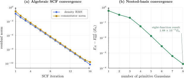
Two independent convergence questions. (a) In the fixed eight-function basis, the density change and commutator residual decrease during undamped SCF iteration. (b) Fully converged energies in nested basis spaces approach a separate high-precision Hartree–Fock reference from above. A tiny SCF residual does not remove the finite-basis error.

Algebraic SCF history

Selected rows from the eight-function run are:

iteration	$E^{(n)}/E_{\mathrm h}$	density RMS	commutator norm
1	$-2.860129704914391$	$4.32\times10^{-2}$	$1.34\times10^{-1}$
2	$-2.861460315274320$	$7.07\times10^{-3}$	$1.64\times10^{-2}$
4	$-2.861492144292867$	$2.85\times10^{-4}$	$5.12\times10^{-4}$
8	$-2.861492180485913$	$3.92\times10^{-7}$	$6.12\times10^{-7}$
12	$-2.861492180485973$	$5.05\times10^{-10}$	$7.81\times10^{-10}$
16	$-2.861492180485971$	$5.82\times10^{-13}$	$1.94\times10^{-12}$

The displayed energy has reached its binary64 plateau before the density criterion passes. Energy changes at the last iterations fluctuate at the scale of a few units in the last printed digit. Continuing to demand smaller energy changes would measure floating-point noise rather than physical accuracy.

The final rebuild and eigensolve give

$$\begin{aligned} \lVert FPS-SPF\rVert_{\mathrm F} &= 5.28\times10^{-13}, \\ \lVert F\mathbf C -\epsilon S\mathbf C \rVert_2 &= 1.14\times10^{-13}. \end{aligned}$$

Nested-basis history

Every row below is separately converged in the SCF sense.

$K$	newly available exponent	$E_K/E_{\mathrm h}$	$E_K-E_{\mathrm{HF}}^{\mathrm{ref}}$	$\kappa(S)$
1	$0.6$	$-2.270271041423163$	$5.9141\times10^{-1}$	$1.00$
2	$1.8$	$-2.537760269411163$	$3.2392\times10^{-1}$	$9.31$
3	$0.2$	$-2.655841263632368$	$2.0584\times10^{-1}$	$34.63$
4	$5.4$	$-2.804954077803264$	$5.6726\times10^{-2}$	$77.73$
5	$16.2$	$-2.848694557217044$	$1.2985\times10^{-2}$	$130.82$
6	$48.6$	$-2.858911600655198$	$2.7684\times10^{-3}$	$185.42$
7	$145.8$	$-2.861059890798204$	$6.2010\times10^{-4}$	$236.22$
8	$437.4$	$-2.861492180485973$	$1.8782\times10^{-4}$	$280.95$

The energy decreases monotonically because the spaces are nested and each SCF solution is the lowest closed-shell solution found in this simple problem. In a more complicated system, a numerical SCF sequence can switch between stationary solutions, break symmetry, or converge to a saddle. A monotone basis table should not be assumed without checking state identity and stability.

Final component ledger

For $K=8$:

component	value in $E_{\mathrm h}$
kinetic energy	$+2.862113233196523$
electron–nucleus energy	$-6.749632049521271$
electron–electron energy	$+1.026026635838774$
total electronic energy	$-2.861492180485973$
occupied orbital energy	$-0.917732772323599$

The component sum is

$$T+V_{\mathrm{en}}+V_{\mathrm{ee}} = E_{\mathrm{RHF}}^{(8)}$$

to floating-point precision.

Because the exponents were not variationally optimized as continuous parameters, the exact Coulomb virial identity need not hold in this fixed basis. The virial defect is

$$2T+V_{\mathrm{en}}+V_{\mathrm{ee}} \approx 6.21\times10^{-4}E_{\mathrm h}.$$

This is a useful diagnostic, but it is not an SCF stopping criterion.

Three Different Error Questions

The phrase “the Hartree–Fock calculation converged” is incomplete. At least three limits must be separated.

SCF iteration error

At fixed basis and fixed occupations, this asks whether

$$P_{\mathrm{out}}[P]-P \approx0.$$

Density changes, commutator norms, orbital-gradient residuals, and energy changes diagnose this error. The final run has reduced it far below the basis error.

One-electron basis error

This asks whether the finite orbital space is flexible enough within the Hartree–Fock model. Using the retained high-precision reference

$$E_{\mathrm{HF}}^{\mathrm{ref}} = -2.861\,679\,995\,612\,239E_{\mathrm h},$$

the eight-function basis error is

$$\Delta_{\mathrm{basis}} = E_{\mathrm{RHF}}^{(8)} -E_{\mathrm{HF}}^{\mathrm{ref}} = 1.878\,151\,262\,660\times10^{-4}E_{\mathrm h}.$$

This value is approximately $1.65\times10^{9}$ times larger than the final generalized eigenpair residual when both are compared as raw numerical magnitudes in atomic units. Solver precision is not basis completeness.

Hartree–Fock model error

The nonrelativistic clamped-nucleus ground-state reference used here is

$$E_{\mathrm{exact}}^{\mathrm{ref}} = -2.903\,724\,377\,034\,120E_{\mathrm h}.$$

The Hartree–Fock correlation-energy magnitude for this Hamiltonian is

$$\begin{aligned} |E_{\mathrm c}^{\mathrm{HF}}| &= E_{\mathrm{HF}}^{\mathrm{ref}} -E_{\mathrm{exact}}^{\mathrm{ref}} \\ &= 0.042\,044\,381\,421\,881E_{\mathrm h}. \end{aligned}$$

The finite-basis-to-exact gap is slightly larger:

$$\begin{aligned} E_{\mathrm{RHF}}^{(8)} -E_{\mathrm{exact}}^{\mathrm{ref}} &= 0.042\,232\,196\,548\,147E_{\mathrm h} \\ &= \Delta_{\mathrm{basis}} +|E_{\mathrm c}^{\mathrm{HF}}|. \end{aligned}$$

Calling the entire finite-basis gap “correlation energy” would include the remaining orbital-basis error.

Relation to the effective-charge notebook

The one-parameter exponential calculation gives

$$E_{\zeta_*} = -2.847\,656\,25E_{\mathrm h}.$$

It is already a closed-shell single-determinant trial state. The present eight-Gaussian Hartree–Fock result lowers that energy by

$$E_{\zeta_*}-E_{\mathrm{RHF}}^{(8)} = 0.013\,835\,930\,485\,973E_{\mathrm h}.$$

That improvement comes from greater flexibility in the occupied orbital, not from electron correlation. Both states use one doubly occupied spatial orbital.

Orbital-Energy Interpretation

The final occupied canonical energy is

$$\epsilon_{\mathrm{occ}} = -0.917\,732\,772\,323\,599E_{\mathrm h}.$$

It is the Lagrange multiplier associated with normalization of the occupied orbital and the eigenvalue of the self-consistent Fock operator in the finite basis. It is not the energy “owned” by one electron.

Why the total is not the orbital sum

For helium,

$$\epsilon_{\mathrm{occ}} = h_\phi+J_\phi,$$

so summing over the two occupied spin-orbitals gives

$$2\epsilon_{\mathrm{occ}} = 2h_\phi+2J_\phi.$$

The actual determinant energy is

$$E_{\mathrm{RHF}} = 2h_\phi+J_\phi.$$

Therefore,

$$E_{\mathrm{RHF}} = 2\epsilon_{\mathrm{occ}}-J_\phi.$$

The Coulomb contribution appears in both one-electron Fock eigenvalues and must be counted only once in the total energy.

Koopmans-style statement

In a fixed-orbital Hartree–Fock picture, removing an electron from an occupied canonical orbital suggests

$$I_{\mathrm{frozen}} \approx -\epsilon_{\mathrm{occ}}.$$

For this run the value is about $0.917733E_{\mathrm h}$. This is not a validated helium ionization energy:

• the cationic orbital is not allowed to relax;
• the basis is incomplete;
• correlation differs between neutral helium and He$^+$;
• finite nuclear mass, relativistic, radiative, and nuclear effects are not included;
• and the program does not perform a matched-basis energy difference.

A proper $\Delta$SCF calculation would solve both charge states with declared models and compare total energies. An experimental ionization threshold requires still more corrections.

Orbitals are representation-dependent

Canonical orbitals diagonalize the occupied–occupied and virtual–virtual Fock blocks, but unitary rotations within an occupied subspace leave the determinant and density unchanged. Helium has only one occupied spatial orbital, so this particular freedom is only an overall phase. In larger systems, orbital shapes and individual orbital energies should not be treated as unique observables.

Validation Ledger

The run is accepted only when all retained checks pass.

Check	Identity or threshold	final result
overlap normalization	$\mathbf C^{\mathsf T}S\mathbf C=1$	error $2.89\times10^{-15}$
electron count	$\operatorname{Tr}(PS)=2$	error $6.22\times10^{-15}$
metric idempotency	$PSP=2P$	norm $4.41\times10^{-15}$
ERI symmetry	required permutations agree	max error $1.78\times10^{-15}$
Fock commutator	$\lVert FPS-SPF\rVert_{\mathrm F}$	$5.28\times10^{-13}$
generalized eigenpair	$\lVert F\mathbf C-\epsilon S\mathbf C\rVert_2$	$1.14\times10^{-13}$
energy identity	$E=2h_\phi+J_\phi$	error $8.88\times10^{-16}E_{\mathrm h}$
orbital identity	$\epsilon=h_\phi+J_\phi$	error $1.11\times10^{-16}E_{\mathrm h}$
double counting	$E=2\epsilon-J_\phi$	error $8.88\times10^{-16}E_{\mathrm h}$
basis ordering	$E_{K+1}\leq E_K$	largest change $-4.32\times10^{-4}E_{\mathrm h}$
HF upper bound	$E_K\geq E_{\mathrm{HF}}^{\mathrm{ref}}$	passed
exact upper bound	$E_K\geq E_{\mathrm{exact}}^{\mathrm{ref}}$	passed

No one check substitutes for all the others. A transposed exchange contraction can preserve matrix symmetry while producing the wrong energy. A density can have the correct trace while failing idempotency. A converged generalized eigenpair can solve the wrong Fock matrix exactly.

What is not independently validated

The notebook does not independently rederive the literature benchmark values. They are retained comparison data with source DOIs in the metadata. It also does not:

• compare each analytic integral against numerical quadrature;
• test displaced or higher-angular-momentum Gaussians;
• prove that no other SCF stationary point exists;
• perform a Hartree–Fock stability analysis;
• optimize the Gaussian exponents;
• or validate properties other than energies and algebraic invariants.

Those are meaningful extensions rather than hidden claims.

Numerical Failure Modes

Energy convergence without density convergence

Near a stationary point, the energy can change quadratically while orbital or density errors change linearly. A tiny $\Delta E$ can therefore coexist with a material density residual. This run requires both criteria and records the commutator independently.

Density convergence to the wrong state

SCF equations can have multiple stationary solutions. A small residual proves self-consistency, not global minimality or physical relevance. Occupation, symmetry, spin contamination, stability, and continuity along a parameter scan must be checked in larger calculations.

Linear dependence

Diffuse or redundant functions can make $S$ nearly singular. Blindly applying $S^{-1/2}$ then magnifies noise. Inspect overlap eigenvalues, remove redundant directions according to a declared threshold, and verify that observables are stable to that threshold.

Incorrect exchange indices

The Coulomb and exchange contractions differ only by an index permutation:

$$J_{\mu\nu} = \sum_{\lambda\sigma} P_{\lambda\sigma} (\mu\nu|\lambda\sigma),$$ $$K_{\mu\nu} = \sum_{\lambda\sigma} P_{\lambda\sigma} (\mu\lambda|\nu\sigma).$$

An implementation should state its integral convention and test an energy identity that depends on exchange, not merely inspect plausible-looking matrix entries.

Reusing a stale Fock matrix

If the energy is evaluated using $P^{(n+1)}$ but $F[P^{(n)}]$, the reported quantity is not the stationary energy functional of either density. The program rebuilds a self-Fock from every output density before computing the recorded energy.

Comparing unmatched Hamiltonians

A finite-nuclear-mass energy, a relativistic energy, an experimental ionization threshold, and the clamped-nucleus nonrelativistic electronic energy are different quantities. More digits do not make them directly comparable.

Downloadable Program and Data

• Download the Python program
• Download the nested-basis convergence CSV
• Download the final SCF history CSV
• Download the two-function matrices JSON
• Download the run metadata JSON

Run the downloaded program from the folder where you saved it:

python hartree-fock-helium.py --output-dir results

The program requires Python with NumPy. It has no network access, random sampling, hidden input files, or platform-specific numerical data.

Artifact roles

Artifact	Role
Python program	canonical executable implementation and validation logic
basis CSV	energies, components, residuals, conditioning, and benchmark gaps for $K=1,\ldots,8$
SCF CSV	iteration-by-iteration energy, density change, and commutator for $K=8$
matrices JSON	complete auditable matrices and identities for $K=2$
metadata JSON	model, tolerances, environment, reference provenance, and pass/fail ledger
SVG figure	visual comparison of algebraic and representation convergence

The JSON matrix artifact is deliberately separate from prose-rounded values. Use it when checking matrix products numerically.

Reproducibility Metadata

The retained run records:

Field	Recorded value
Python	3.12.13
NumPy	2.3.5
platform	Windows 11, x86-64
floating-point type	NumPy float64
density tolerance	$10^{-12}$
energy tolerance	$10^{-13}E_{\mathrm h}$
random seed	none
program license	MIT
Hartree–Fock reference DOI	10.2477/jccjie.2024-0032
exact nonrelativistic reference DOI	10.1002/qua.10344

The four generated data files were reproduced twice with identical SHA-256 hashes in the retained environment. Deterministic equality on one platform is strong evidence about the workflow, but cross-platform BLAS or eigensolver differences can change the last few floating-point digits without changing the scientific conclusion.

Common Mistakes

Calling an SCF tolerance an energy error bar

The threshold controls termination of an iterative solver. It does not bound basis error, model error, or property error.

Solving an ordinary eigenproblem

Primitive Gaussian coefficients satisfy $F C=S C\epsilon$. Ignoring $S$ changes both normalization and the stationary equation.

Omitting the occupation factor

For one doubly occupied spatial orbital,

$$P_{\mu\nu}=2C_\mu C_\nu.$$

Dropping the factor of two gives the wrong electron count and Fock field.

Doubling orbital energies

$2\epsilon_{\mathrm{occ}}$ double counts the Coulomb interaction. The total energy requires the density-functional expression or the equivalent $2\epsilon_{\mathrm{occ}}-J_\phi$ identity.

Calling all of the exact-energy gap correlation

Only the complete-basis Hartree–Fock-to-exact difference defines the usual Hartree–Fock correlation energy for a specified Hamiltonian. A finite-basis gap also contains basis error.

Assuming Gaussian coefficients are probabilities

The primitives are nonorthogonal. Individual $C_\mu^2$ values are not basis-independent occupation probabilities, and their sum need not be one. Normalization uses $\mathbf C^{\mathsf T}S\mathbf C$.

Interpreting the coefficient sign

The overall sign of an eigenvector is arbitrary. A sign flip of all occupied coefficients changes no density or observable.

Trusting monotone energy alone

Monotone values can still come from incorrect integrals or a consistently wrong functional. Independent algebraic identities and benchmark comparisons remain necessary.

Treating a Gaussian benchmark as a production basis

The exponent list is an instructional nested sequence. It has no standard basis-set name, contraction error analysis, polarization hierarchy, or property-specific optimization.

Treating minus the orbital energy as an exact ionization energy

Koopmans’ relation freezes orbitals and remains inside Hartree–Fock. Relaxation, correlation, basis error, and physical corrections all matter for comparison with a measured threshold.

Extensions

Optimize Gaussian exponents

Treat the exponents as nonlinear variational parameters while preserving positivity and avoiding near-linear dependence. This should lower the finite-basis energy, but every optimization must rerun SCF to convergence. The outer and inner tolerances should be reported separately.

Numerical radial Hartree–Fock

Replace the Gaussian expansion by a radial grid, finite elements, B-splines, or a complete exponential-type basis. Compare energy, density, cusp behavior, and radial moments, not only the total energy.

Matched-basis delta SCF

Solve He and He$^+$ with compatible basis and Hamiltonian choices, then form

$$I_{\Delta\mathrm{SCF}} = E_{\mathrm{HF}}(\mathrm{He}^+) -E_{\mathrm{HF}}(\mathrm{He}).$$

Compare this relaxed Hartree–Fock value with the frozen-orbital estimate $-\epsilon_{\mathrm{occ}}$.

More occupied orbitals

Be or Ne introduces multiple occupied spatial orbitals and makes same-spin exchange among distinct orbitals explicit. It also introduces more possibilities for slow convergence, occupation changes, and orbital rotations.

Molecular centres

Moving basis functions to more than one nucleus requires nuclear-repulsion energy and geometry conventions. For molecular Gaussian Hartree–Fock it also requires the Gaussian product theorem, Boys functions, and more general electron-repulsion integrals. Molecular Orbital Computation isolates the preceding LCAO bridge in a one-electron, two-centre Slater-basis problem, where overlap and nuclear repulsion are already unavoidable but self-consistency and electron-repulsion integrals are absent.

Post-Hartree–Fock correlation

Configuration interaction, many-body perturbation theory, coupled-cluster methods, and explicitly correlated approaches enlarge the many-electron trial space beyond one determinant. Basis convergence and correlation convergence remain separate questions there as well.

Exercises

Exercise 1: Normalize a primitive Gaussian

Show that

$$\chi_\alpha(\mathbf r) = \left( \frac{2\alpha}{\pi} \right)^{3/4} e^{-\alpha r^2}$$

is normalized in three dimensions.

Solution

The squared norm is

$$\int_{\mathbb R^3} |\chi_\alpha(\mathbf r)|^2\,d^3r = N_\alpha^2 \int_{\mathbb R^3} e^{-2\alpha r^2}\,d^3r.$$

Use the three-dimensional Gaussian integral

$$\int_{\mathbb R^3} e^{-\beta r^2}\,d^3r = \left( \frac{\pi}{\beta} \right)^{3/2}.$$

Then

$$\int |\chi_\alpha|^2\,d^3r = N_\alpha^2 \left( \frac{\pi}{2\alpha} \right)^{3/2}.$$

Setting this equal to one gives

$$N_\alpha^2 = \left( \frac{2\alpha}{\pi} \right)^{3/2},$$

and taking the positive square root yields the stated normalization.

Exercise 2: Derive the overlap formula

Starting from two normalized same-centre primitives with exponents $\alpha_\mu$ and $\alpha_\nu$, derive $S_{\mu\nu}$. Verify that $S_{\mu\mu}=1$.

Solution

The product is

$$\chi_\mu(\mathbf r)\chi_\nu(\mathbf r) = N_\mu N_\nu e^{-(\alpha_\mu+\alpha_\nu)r^2}.$$

With $p_{\mu\nu}=\alpha_\mu+\alpha_\nu$,

$$S_{\mu\nu} = N_\mu N_\nu \int_{\mathbb R^3} e^{-p_{\mu\nu}r^2}\,d^3r = N_\mu N_\nu \left( \frac{\pi}{p_{\mu\nu}} \right)^{3/2}.$$

For $\mu=\nu$, $p_{\mu\mu}=2\alpha_\mu$ and

$$\begin{aligned} S_{\mu\mu} &= \left( \frac{2\alpha_\mu}{\pi} \right)^{3/2} \left( \frac{\pi}{2\alpha_\mu} \right)^{3/2} \\ &=1. \end{aligned}$$

Exercise 3: Prove symmetric orthogonalization

Let $S=UsU^{\mathsf T}$ with orthogonal $U$ and positive diagonal $s$. Show that $X=Us^{-1/2}U^{\mathsf T}$ obeys $X^{\mathsf T}SX=I$, and derive the transformed Fock equation.

Solution

Because $S$ and $X$ are symmetric,

$$\begin{aligned} X^{\mathsf T}SX &= \left( Us^{-1/2}U^{\mathsf T} \right) \left( UsU^{\mathsf T} \right) \left( Us^{-1/2}U^{\mathsf T} \right). \end{aligned}$$

Using the declared decomposition,

$$\begin{aligned} X^{\mathsf T}SX &= Us^{-1/2} \left( U^{\mathsf T}U \right) s \left( U^{\mathsf T}U \right) s^{-1/2}U^{\mathsf T} \\ &= U I U^{\mathsf T} \\ &=I. \end{aligned}$$

Write $\mathbf C=X\widetilde{\mathbf C}$ in

$$F\mathbf C=S\mathbf C\epsilon.$$

Premultiplying by $X^{\mathsf T}$ gives

$$X^{\mathsf T}FX\widetilde{\mathbf C} = X^{\mathsf T}SX\widetilde{\mathbf C}\epsilon = \widetilde{\mathbf C}\epsilon.$$

Thus the transformed problem is an ordinary symmetric eigenproblem.

Exercise 4: Check the metric density identities

For $P=2\mathbf C\mathbf C^{\mathsf T}$ and $\mathbf C^{\mathsf T}S\mathbf C=1$, prove

$$\operatorname{Tr}(PS)=2$$

and

$$PSP=2P.$$

Solution

Use cyclicity of the trace:

$$\begin{aligned} \operatorname{Tr}(PS) &= 2\operatorname{Tr} \left( \mathbf C\mathbf C^{\mathsf T}S \right) \\ &= 2\operatorname{Tr} \left( \mathbf C^{\mathsf T}S\mathbf C \right) \\ &=2. \end{aligned}$$

For idempotency,

$$\begin{aligned} PSP &= \left( 2\mathbf C\mathbf C^{\mathsf T} \right) S \left( 2\mathbf C\mathbf C^{\mathsf T} \right) \\ &= 4\mathbf C \left( \mathbf C^{\mathsf T}S\mathbf C \right) \mathbf C^{\mathsf T} \\ &= 4\mathbf C\mathbf C^{\mathsf T} \\ &=2P. \end{aligned}$$

The factor of two reflects double occupation. For an orthonormal spin-orbital projector with unit occupations, the corresponding idempotency convention would differ.

Exercise 5: Audit the minimal coefficient vector

Using the rounded two-function values, estimate $\mathbf C^{\mathsf T}S\mathbf C$ and explain why $C_1^2+C_2^2$ is not the normalization test.

Solution

With

$$\mathbf C \approx \begin{pmatrix} -0.679571\\ -0.367816 \end{pmatrix}$$

and $S_{12}=S_{21}\approx0.805927$,

$$\begin{aligned} \mathbf C^{\mathsf T}S\mathbf C &= C_1^2+C_2^2+2S_{12}C_1C_2 \\ &\approx 0.4618+0.1353+0.4029 \\ &\approx1.0000. \end{aligned}$$

By contrast,

$$C_1^2+C_2^2 \approx 0.5971.$$

The missing cross term is large because the basis functions overlap strongly. Coefficient squares can be interpreted as ordinary component weights only after transforming to an orthonormal basis, and even then those weights remain representation-dependent.

Exercise 6: Derive the double-counting identity

For a two-electron closed shell, use

$$E=2h_\phi+J_\phi$$

and

$$\epsilon=h_\phi+J_\phi$$

to express the total energy in terms of $\epsilon$ and $J_\phi$. Evaluate the identity for the minimal demonstrator.

Solution

Twice the orbital energy is

$$2\epsilon = 2h_\phi+2J_\phi.$$

Subtract one Coulomb integral:

$$2\epsilon-J_\phi = 2h_\phi+J_\phi = E.$$

Using the retained values,

$$\begin{aligned} 2\epsilon-J_\phi &= 2(-0.733\,025\,588\,080) -1.071\,709\,093\,252 \\ &= -2.537\,760\,269\,412E_{\mathrm h}, \end{aligned}$$

where the last displayed digit differs from the full-precision stored result because the inputs were rounded in the page. The JSON artifact verifies the identity to approximately $9\times10^{-16}E_{\mathrm h}$.

Exercise 7: Separate the error budget

Using

$$\begin{aligned} E_8 &= -2.861492180485973E_{\mathrm h}, \\ E_{\mathrm{HF}}^{\mathrm{ref}} &= -2.861679995612239E_{\mathrm h}, \\ E_{\mathrm{exact}}^{\mathrm{ref}} &= -2.903724377034120E_{\mathrm h}, \end{aligned}$$

compute the finite-basis error, Hartree–Fock correlation-energy magnitude, and total finite-basis-to-exact gap. Check the additive relation.

Solution

The basis error is

$$\Delta_{\mathrm{basis}} = E_8-E_{\mathrm{HF}}^{\mathrm{ref}} = 0.000187815126266E_{\mathrm h}.$$

The Hartree–Fock correlation-energy magnitude is

$$|E_{\mathrm c}^{\mathrm{HF}}| = E_{\mathrm{HF}}^{\mathrm{ref}} -E_{\mathrm{exact}}^{\mathrm{ref}} = 0.042044381421881E_{\mathrm h}.$$

The total gap is

$$E_8-E_{\mathrm{exact}}^{\mathrm{ref}} = 0.042232196548147E_{\mathrm h}.$$

Indeed,

$$0.000187815126266 +0.042044381421881 = 0.042232196548147.$$

The calculation shows why the finite-basis-to-exact gap cannot be labeled pure correlation energy.

Exercise 8: Explain the Gaussian cusp failure

Show that any finite linear combination

$$\phi(r) = \sum_{\mu=1}^{K} C_\mu e^{-\alpha_\mu r^2}$$

has $\phi'(0)=0$. Contrast this with the electron–nucleus cusp condition for a Coulombic $s$ orbital.

Solution

Differentiate term by term:

$$\phi'(r) = \sum_{\mu=1}^{K} -2\alpha_\mu r C_\mu e^{-\alpha_\mu r^2}.$$

Every term contains a factor of $r$, so

$$\phi'(0)=0.$$

For a Coulombic nucleus, the spherical-average electron–nucleus cusp condition has the form

$$\left. \frac{\phi'(r)}{\phi(r)} \right|_{r=0} = -Z$$

for a one-electron $s$ orbital, with the corresponding many-electron statement applied to the wavefunction as one electron approaches the nucleus. For $Z>0$ and $\phi(0)\neq0$, the exact derivative is nonzero. Therefore no finite same-centre Gaussian sum satisfies the cusp exactly.

Increasing the number of tight Gaussians can approximate the orbital and its energy well away from the exact pointwise cusp, but it does not change this analytic fact.

Exercise 9: Design a safer stopping rule

Suppose an SCF run reaches $|\Delta E|<10^{-12}E_{\mathrm h}$ while its commutator norm remains $10^{-4}$. Should it be accepted? Propose a stopping and diagnosis policy.

Solution

It should not be accepted as a self-consistent solution. Near a stationary point, an energy can be insensitive to an orbital displacement even when the orbital gradient remains significant. A commutator norm of $10^{-4}$ is incompatible with a tightly converged occupied subspace.

A practical policy is to require all of:

$$|\Delta E|<\tau_E, \qquad \operatorname{RMS}(\Delta P)<\tau_P, \qquad \lVert FPS-SPF\rVert_{\mathrm F}<\tau_R.$$

The thresholds should be chosen relative to the desired observable accuracy and reported with the result. If energy appears converged but $R$ stalls:

1. inspect occupations and overlap conditioning;
2. verify that energy and residual use the same output density;
3. try damping or DIIS while retaining the residual test;
4. test a different initial guess;
5. perform stability analysis where available;
6. and distinguish solver failure from a basis or symmetry problem.

An accelerator can reduce the residual, but it cannot turn an incorrect Fock construction into the correct equations.

Key Takeaways

• Hartree–Fock is nonlinear because the one-electron operator depends on the occupied density that solves it.
• A nonorthogonal basis requires $FC=SC\epsilon$, metric normalization, and metric-aware density identities.
• Fock eigenvalues contain two-electron fields; their occupied sum is not the total electronic energy.
• SCF residuals, basis convergence, and correlation error answer different questions.
• A flexible single orbital lowers the effective-charge result without adding electron correlation.
• Gaussian integrals can be exact while the Gaussian representation remains incomplete and cusp-deficient.
• Reproducibility requires matrices, iteration history, tolerances, reference provenance, and independent algebraic checks.

Cross-Links

• Computational AMO and Quantum Chemistry
• Computational Atomic Structure
• Variational Helium Notebook
• Molecular Orbital Computation
• Helium Atom
• Hartree Method
• Hartree–Fock for Atoms
• Exchange and Correlation
• Hartree–Fock Approximation
• Variational Principle
• Eigenvalues and Eigenvectors
• Atomic Units
• Notebook Index

References

1. C. C. J. Roothaan, “New Developments in Molecular Orbital Theory,” Reviews of Modern Physics 23, 69–89 (1951), doi:10.1103/RevModPhys.23.69.
2. G. G. Hall, “The Molecular Orbital Theory of Chemical Valency. VIII. A Method of Calculating Ionization Potentials,” Proceedings of the Royal Society A 205, 541–552 (1951), doi:10.1098/rspa.1951.0048.
3. S. F. Boys, “Electronic Wave Functions. I. A General Method of Calculation for the Stationary States of Any Molecular System,” Proceedings of the Royal Society A 200, 542–554 (1950), doi:10.1098/rspa.1950.0036.
4. P. Pulay, “Convergence Acceleration of Iterative Sequences. The Case of SCF Iteration,” Chemical Physics Letters 73, 393–398 (1980), doi:10.1016/0009-2614(80)80396-4.
5. Y. Hatano and S. Yamamoto, “Accuracy of Hartree–Fock Energies and Physical Properties Calculated Using Lambda Functions for Helium, Lithium, and Beryllium Atoms,” Journal of Computer Chemistry, Japan – International Edition 11, article 2024-0032 (2025), doi:10.2477/jccjie.2024-0032.
6. J. S. Sims and S. A. Hagstrom, “High-Precision Hy–CI Variational Calculations for the Ground State of Neutral Helium and Helium-Like Ions,” International Journal of Quantum Chemistry 90, 1600–1609 (2002), doi:10.1002/qua.10344.
7. T. Kato, “On the Eigenfunctions of Many-Particle Systems in Quantum Mechanics,” Communications on Pure and Applied Mathematics 10, 151–177 (1957), doi:10.1002/cpa.3160100201.
8. P.-O. Löwdin, “Correlation Problem in Many-Electron Quantum Mechanics. I,” Advances in Chemical Physics 2, 207–322 (1959), doi:10.1002/9780470143599.ch2.
9. A. Szabo and N. S. Ostlund, Modern Quantum Chemistry: Introduction to Advanced Electronic Structure Theory, Dover (1996).
10. T. Helgaker, P. Jørgensen, and J. Olsen, Molecular Electronic-Structure Theory, Wiley (2000), doi:10.1002/9781119019572.
11. C. Froese Fischer, T. Brage, and P. Jönsson, Computational Atomic Structure: An MCHF Approach, Institute of Physics Publishing (1997).
12. W. R. Johnson, Atomic Structure Theory: Lectures on Atomic Physics, Springer (2007), doi:10.1007/978-3-540-68013-0.

Further Study

The Molecular Orbital Computation page moves the same overlap and generalized-eigenvalue discipline to two centres. Its one-electron H₂⁺ model introduces bonding and antibonding combinations, nuclear repulsion, and geometry dependence while preserving the distinction among solver, basis, and model convergence. A molecular Gaussian Hartree–Fock implementation is the subsequent step; that is where the Gaussian product theorem and multicentre electron-repulsion integrals enter.