Molecular Orbital Computation

This notebook turns the smallest molecular orbital problem into a complete matrix computation. Two normalized hydrogenic $1s$ functions, one on each proton of H$_2^+$, form a nonorthogonal basis. The program evaluates their analytic matrix elements, solves

$$H\mathbf c = \epsilon S\mathbf c$$

at 291 internuclear separations, identifies the gerade and ungerade eigenvectors by symmetry, adds proton–proton repulsion, locates the variational minimum, and writes the orbitals’ bond-axis densities.

At $R=2a_0$, numerical generalized diagonalization gives

$$\begin{aligned} U_g &= -0.553\,771\,495\,318\,482E_{\mathrm h}, \\ U_u &= -0.160\,853\,965\,596\,687E_{\mathrm h}. \end{aligned}$$

The numerical eigenvalues agree with the symmetry-adapted closed forms to at most $1.11\times10^{-15}E_{\mathrm h}$ over the retained grid. The smallest residuals do not make the minimal basis quantitatively accurate: its ground curve has a minimum

$$U_g^{\mathrm{LCAO}}(R_e) = -0.564\,830\,992\,370\,808E_{\mathrm h}$$

at

$$R_e^{\mathrm{LCAO}} = 2.492\,830\,425\,253a_0,$$

whereas a high-precision Born–Oppenheimer reference is substantially deeper and shorter.

Run the investigation. The program and retained results below support the stated experiment. Follow Running an Experiment for environment and output-directory guidance. The recorded evidence applies to its stated parameters and environment.

Canonical Scope

H₂⁺ Ion owns the exact two-centre Coulomb problem, prolate-spheroidal separation, analytic derivation of the minimal-LCAO integrals, parity-state physics, long-range structure, and accurate spectroscopy. Molecular Orbitals owns the general LCAO formalism, molecular symmetry labels, orbital diagrams, occupations, localized-orbital freedom, and many-electron interpretation. Potential Energy Surfaces owns the broader meaning of molecular potentials, forces, stationary geometries, and nuclear dynamics.

This page owns the reproducible finite-matrix experiment:

• assemble $S(R)$ and $H(R)$ from declared analytic inputs;
• solve the nonorthogonal problem by symmetric orthogonalization;
• classify and phase-fix numerical eigenvectors;
• test them against independent symmetry-adapted formulas;
• keep electronic and total molecular energies in separate columns;
• scan bonding and antibonding curves on a declared grid;
• locate a continuous variational minimum outside that grid;
• sample bonding and antibonding densities along the molecular axis;
• compare solver error, basis error, and physical-model scope;
• and retain matrices, curves, densities, metadata, and validation results.

The integral formulas are stated because they are executable inputs, but their full coordinate-space derivation remains at the canonical H$_2^+$ page.

Reproducibility Contract

Item	Notebook choice
system	H$_2^+$, two protons and one electron
nuclear treatment	clamped protons at separation $R$
electronic Hamiltonian	nonrelativistic two-centre Coulomb Hamiltonian
one-electron basis	normalized hydrogenic $1s$ Slater orbital on each proton
orbital exponent	fixed at $\zeta=1a_0^{-1}$
matrix size	$2\times2$
eigensolver	symmetric orthogonalization plus a real symmetric eigensolve
curve grid	291 points, $0.5\leq R/a_0\leq15$
minimum search	golden-section search on $1\leq R/a_0\leq5$
density sample	bond axis, $R=2a_0$, 401 points on $-5\leq z/a_0\leq5$
arithmetic	IEEE 754 binary64 through NumPy
randomness	none
artifacts	Python program, two CSV files, two JSON files, SVG figure

This is a one-electron calculation. There is no electron–electron interaction, SCF loop, exchange field, or correlation approximation. “Molecular orbital” is an exact one-electron concept for the specified finite matrix problem even though the two-function spatial representation is approximate.

Hamiltonian and Energy Conventions

Place protons $A$ and $B$ at

$$\mathbf R_A = -\frac{R}{2}\mathbf e_z, \qquad \mathbf R_B = +\frac{R}{2}\mathbf e_z.$$

With

$$r_A = |\mathbf r-\mathbf R_A|, \qquad r_B = |\mathbf r-\mathbf R_B|,$$

the clamped-proton electronic Hamiltonian in atomic units is

$$h_e(R) = -\frac12\nabla^2 -\frac{1}{r_A} -\frac{1}{r_B}.$$

The finite-basis generalized eigenvalue $\epsilon_n(R)$ is an electronic energy. Nuclear motion instead sees the Born–Oppenheimer curve

$$U_n(R) = \epsilon_n(R)+\frac{1}{R}.$$

The $1/R$ term is constant with respect to the electron coordinate, so it does not change electronic eigenvectors. It does change the curve shape, equilibrium geometry, well depth, and short-range limit.

Three quantities in the output

CSV quantity	Definition	Limit as $R\to\infty$
electronic_g_Eh	$\epsilon_g(R)$	$-1/2$ plus the remote-proton attraction before cancellation
total_g_Eh	$U_g(R)=\epsilon_g(R)+1/R$	$-1/2$
splitting_Eh	$U_u-U_g=\epsilon_u-\epsilon_g$	$0$

At finite $R$, the electronic and total energies must not be interchanged. At $R=2a_0$, proton–proton repulsion is

$$\frac1R = 0.5E_{\mathrm h}.$$

That is why the ground electronic eigenvalue $-1.0537714953E_{\mathrm h}$ corresponds to a total curve value of only $-0.5537714953E_{\mathrm h}$.

Basis Functions

The retained basis consists of

$$\phi_A(\mathbf r) = \frac{e^{-r_A}}{\sqrt\pi}, \qquad \phi_B(\mathbf r) = \frac{e^{-r_B}}{\sqrt\pi}.$$

Each function is normalized:

$$\langle\phi_A|\phi_A\rangle = \langle\phi_B|\phi_B\rangle = 1.$$

They are not mutually orthogonal. Their overlap is

$$S_{AB}(R) = \langle\phi_A|\phi_B\rangle \equiv S(R).$$

The orbital expansion is

$$\psi(\mathbf r;R) = c_A\phi_A(\mathbf r) +c_B\phi_B(\mathbf r).$$

Normalization therefore means

$$\mathbf c^{\mathsf T}S\mathbf c = c_A^2+c_B^2+2S c_Ac_B = 1,$$

not $c_A^2+c_B^2=1$.

What is fixed and what varies

The proton separation $R$ varies. The basis centres move with the protons, but the radial exponent remains $\zeta=1$. The functions therefore retain the shape of isolated-hydrogen $1s$ orbitals at every geometry.

This restriction omits two important responses:

• contraction: near equilibrium, the orbital can contract under attraction from both protons;
• polarization: each atom-centred component can deform toward the other proton and acquire higher angular structure.

The minimal basis can represent coherent sharing between centres, but not those deformations. It is a qualitative bonding model and a sharp numerical test, not a spectroscopic basis.

Analytic Matrix Inputs

The notebook uses the dimensionless separation $R/a_0$ as the numerical variable. For the fixed exponent $\zeta=1$, the overlap is

$$S(R) = e^{-R} \left( 1+R+\frac{R^2}{3} \right).$$

Define the Coulomb and resonance integrals

$$J(R) = \left\langle \phi_A \left| -\frac1{r_B} \right| \phi_A \right\rangle$$

and

$$K(R) = \left\langle \phi_A \left| -\frac1{r_A} \right| \phi_B \right\rangle.$$

Their closed forms are

$$J(R) = -\frac1R +e^{-2R} \left( 1+\frac1R \right)$$

and

$$K(R) = -e^{-R}(1+R).$$

Here $K$ is a one-electron resonance integral. It is not the same object as the electron–electron exchange integral often also denoted $K$ in Hartree–Fock theory.

Overlap and Hamiltonian matrices

Homonuclear exchange symmetry gives

$$S(R) = \begin{pmatrix} 1 & S_{AB}\\ S_{AB} & 1 \end{pmatrix}.$$

Using the isolated-hydrogen eigenvalue $-1/2$,

$$H_{AA} = H_{BB} = -\frac12+J,$$

and

$$H_{AB} = H_{BA} = -\frac12S+K.$$

Thus

$$H(R) = \begin{pmatrix} H_{00} & H_{01}\\ H_{01} & H_{00} \end{pmatrix}.$$

The program constructs these matrices afresh at every grid point. It does not hard-code the eigenvalues or eigenvectors.

Generalized Diagonalization

The numerical problem is

$$H\mathbf c_n = \epsilon_n S\mathbf c_n.$$

Because $0<S_{AB}<1$ for every finite positive $R$, the overlap matrix is positive definite. Diagonalize it as

$$S = U s U^{\mathsf T}$$

and define the symmetric orthogonalizer

$$X = U s^{-1/2}U^{\mathsf T}.$$

Then

$$X^{\mathsf T}SX=I,$$

and the transformed problem is

$$\left( X^{\mathsf T}HX \right) \widetilde{\mathbf c}_n = \epsilon_n\widetilde{\mathbf c}_n.$$

The original coefficients are

$$\mathbf c_n = X\widetilde{\mathbf c}_n.$$

The code symmetrizes $X^{\mathsf T}HX$ before calling the Hermitian eigensolver, then checks both

$$\mathbf c_n^{\mathsf T}S\mathbf c_n=1$$

and

$$\left\| H\mathbf c_n -\epsilon_nS\mathbf c_n \right\|_2.$$

Symmetry classification

For identical centres, the numerical vectors must have one of two parity patterns:

$$c_Ac_B>0 \quad\Longrightarrow\quad g,$$ $$c_Ac_B<0 \quad\Longrightarrow\quad u.$$

The program classifies states by this sign product rather than assuming that array column zero is always called “bonding.” It then fixes a display phase: the gerade coefficients have positive sum, and the ungerade coefficient on centre $A$ is positive.

The global phase remains arbitrary. Multiplying either coefficient vector by $-1$ leaves every density, energy, and residual unchanged.

Near-degenerate vectors

At large $R$, the gerade–ungerade splitting becomes small. Eigenvalues remain accurate while individual eigenvectors become more sensitive to roundoff inside the nearly degenerate two-dimensional subspace. Across the retained grid, the largest departure from exact coefficient parity is about

$$2.14\times10^{-11},$$

at $R=14.8a_0$. The largest generalized eigenpair residual is nevertheless only

$$1.42\times10^{-15}.$$

This is not a contradiction. Eigenvector conditioning depends on spectral separation, not only on residual size.

Complete Matrix Example at Two Bohr

At $R=2a_0$, the analytic scalar integrals are

$$\begin{aligned} S &= 0.586\,452\,894\,025\,322, \\ J &= -0.472\,526\,541\,666\,899E_{\mathrm h}, \\ K &= -0.406\,005\,849\,709\,838E_{\mathrm h}. \end{aligned}$$

The retained overlap matrix is

$$S = \begin{pmatrix} 1 & 0.586\,452\,894\,025\,322 \\ 0.586\,452\,894\,025\,322 & 1 \end{pmatrix},$$

and the electronic Hamiltonian is

$$H = \begin{pmatrix} -0.972\,526\,541\,666\,899 & -0.699\,232\,296\,722\,499 \\ -0.699\,232\,296\,722\,499 & -0.972\,526\,541\,666\,899 \end{pmatrix} E_{\mathrm h}.$$

The overlap eigenvalues are $1+S$ and $1-S$, so

$$\kappa(S) = \frac{1+S}{1-S} = 3.836\,208\,429\,717\,46.$$

Gerade state

The numerical coefficient vector is

$$\mathbf c_g = \begin{pmatrix} 0.561\,398\,711\,506\,190 \\ 0.561\,398\,711\,506\,190 \end{pmatrix}.$$

It gives

$$\epsilon_g = -1.053\,771\,495\,318\,482E_{\mathrm h}$$

and

$$U_g = \epsilon_g+\frac12 = -0.553\,771\,495\,318\,482E_{\mathrm h}.$$

The metric norm differs from one by about $9\times10^{-16}$, and the generalized residual is approximately $9.42\times10^{-16}$.

Ungerade state

The numerical coefficient vector is

$$\mathbf c_u = \begin{pmatrix} 1.099\,569\,055\,325\,478 \\ -1.099\,569\,055\,325\,478 \end{pmatrix}.$$

Coefficients larger than one are not a normalization failure. Destructive overlap contributes a negative cross term:

$$\begin{aligned} \mathbf c_u^{\mathsf T}S\mathbf c_u &= 2c^2(1-S) \\ &=1. \end{aligned}$$

The state has

$$\epsilon_u = -0.660\,853\,965\,596\,687E_{\mathrm h}$$

and

$$U_u = -0.160\,853\,965\,596\,687E_{\mathrm h}.$$

Its metric-norm error is about $3\times10^{-16}$, and its generalized residual is approximately $2.00\times10^{-16}$.

Closed-Form Cross-Check

Symmetry predicts the normalized combinations

$$\psi_g = \frac{ \phi_A+\phi_B }{ \sqrt{2(1+S)} },$$ $$\psi_u = \frac{ \phi_A-\phi_B }{ \sqrt{2(1-S)} }.$$

The corresponding electronic energies are

$$\epsilon_g = \frac{ H_{00}+H_{01} }{ 1+S }$$

and

$$\epsilon_u = \frac{ H_{00}-H_{01} }{ 1-S }.$$

The notebook evaluates these expressions separately from the generalized eigensolver and compares them point by point. Over all 291 geometries,

$$\max_R \left| \epsilon_n^{\mathrm{eig}}(R) -\epsilon_n^{\mathrm{sym}}(R) \right| = 1.11\times10^{-15}E_{\mathrm h}.$$

This check is valuable because it tests matrix diagonalization, metric normalization, state assignment, and energy ordering. It does not independently validate the analytic integral formulas; those require either their coordinate-space derivation or a separate quadrature implementation.

Potential Curves and Densities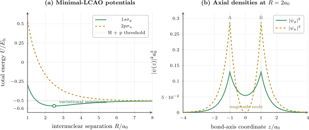

Outputs of the retained two-function H$_2^+$ calculation. (a) The total curves include proton–proton repulsion. The $1s\sigma_g$ curve has a variational well; the fixed-exponent $2p\sigma_u$ curve approaches the H $+$ p threshold from above. (b) At $R=2a_0$, constructive interference leaves nonzero gerade density at the midpoint, whereas the ungerade combination has a symmetry-enforced node. The plotted values sample a three-dimensional density along one line; they are not a one-dimensional marginal probability.

Selected curve values

$R/a_0$	$S$	$U_g/E_{\mathrm h}$	$U_u/E_{\mathrm h}$	$U_u-U_g$
1.0	$0.858385$	$-0.288366$	$+0.545401$	$0.833767$
2.0	$0.586453$	$-0.553771$	$-0.160854$	$0.392918$
2.49283	$0.460026$	$-0.564831$	$-0.289231$	$0.275600$
5.0	$0.096577$	$-0.519203$	$-0.476571$	$0.042633$
10.0	$0.002013$	$-0.500298$	$-0.499701$	$5.96\times10^{-4}$
15.0	$2.78\times10^{-5}$	$-0.500003$	$-0.499997$	$6.08\times10^{-6}$

The short-range rise comes from proton–proton repulsion and localization pressure. At large $R$, the two parity states become nearly degenerate and both approach the separated H $+$ p threshold.

Continuous minimum versus grid minimum

The curve CSV uses a fixed $0.05a_0$ spacing. A grid minimum would therefore quantize the reported geometry. The program instead minimizes the analytic minimal-LCAO curve by golden-section search on

$$1\leq R/a_0\leq5.$$

After 71 bracket updates, it obtains

$$\begin{aligned} R_e^{\mathrm{LCAO}} &= 2.492\,830\,425\,253a_0, \\ U_e^{\mathrm{LCAO}} &= -0.564\,830\,992\,371E_{\mathrm h}, \\ D_e^{\mathrm{LCAO}} &= 0.064\,830\,992\,371E_{\mathrm h}. \end{aligned}$$

The continuous search removes grid-location error, but it does not reduce basis error.

Comparison with an accurate reference

The retained high-precision ground-state comparison is

$$\begin{aligned} R_e^{\mathrm{ref}} &= 1.997\,193\,32a_0, \\ U_e^{\mathrm{ref}} &= -0.602\,634\,619\,1E_{\mathrm h}, \\ D_e^{\mathrm{ref}} &= 0.102\,634\,619\,1E_{\mathrm h}. \end{aligned}$$

The minimal basis recovers

$$\frac{ D_e^{\mathrm{LCAO}} }{ D_e^{\mathrm{ref}} } = 0.631\,667\,881,$$

or about $63.17\%$ of the accurate well depth. Its equilibrium distance is larger by

$$\frac{ R_e^{\mathrm{LCAO}}-R_e^{\mathrm{ref}} }{ R_e^{\mathrm{ref}} } = 0.248\,167,$$

or about $24.82\%$.

The agreement is qualitatively strong and quantitatively poor. It predicts a one-electron covalent bond with the correct symmetry, but not a spectroscopic-quality curve.

Interference Densities

Along the bond axis, the program evaluates the three-dimensional basis functions at

$$\mathbf r=z\mathbf e_z.$$

For nuclei at $z=\pm R/2$,

$$\phi_A(z) = \frac{ e^{-|z+R/2|} }{ \sqrt\pi }, \qquad \phi_B(z) = \frac{ e^{-|z-R/2|} }{ \sqrt\pi }.$$

The numerical orbitals are

$$\psi_n(z) = c_{A,n}\phi_A(z) +c_{B,n}\phi_B(z).$$

At $R=2a_0$ and $z=0$,

$$\phi_A(0)=\phi_B(0),$$

so

$$\psi_u(0)=0$$

by antisymmetry, while

$$|\psi_g(0)|^2 = 0.054\,308\,021\,08a_0^{-3}.$$

The interference term

For real basis functions,

$$|\psi|^2 = c_A^2\phi_A^2 +c_B^2\phi_B^2 +2c_Ac_B\phi_A\phi_B.$$

The cross term is positive for the gerade state and negative for the ungerade state. This is the precise algebra behind constructive and destructive interference in this basis.

The density picture alone is not a complete energy decomposition. Whether bonding stabilization is assigned to kinetic or potential contributions can depend on the variational path and partition. The invariant claims here are the generalized eigenvalues, total curve, parity, node, and variational ordering.

Axis sample is not a marginal density

The CSV column density_g_per_bohr3 has units $a_0^{-3}$ because it is the three-dimensional density evaluated on the line $x=y=0$. Integrating it only over $z$ does not give one:

$$\int_{-\infty}^{\infty} |\psi(0,0,z)|^2\,dz \neq 1.$$

A one-dimensional marginal would require transverse integration:

$$\rho_z(z) = \iint |\psi(x,y,z)|^2\,dx\,dy,$$

for which

$$\int\rho_z(z)\,dz=1.$$

The retained axis file is designed for shape inspection, node tests, and plotting, not population analysis.

Bonding and Antibonding Interpretation

The labels $1s\sigma_g$ and $2p\sigma_u$ combine several statements:

• $\sigma$ means zero orbital-angular-momentum projection about the molecular axis;
• $g$ and $u$ describe inversion parity through the midpoint;
• bonding and antibonding describe the usual effect of constructive or destructive centre mixing in the bonding region;
• the numerical prefix and atomic label identify conventional correlation limits, not exact hydrogenic quantum numbers at every $R$.

What the finite curve proves

The minimal calculation proves that this two-function gerade trial space contains a normalized state below the H $+$ p threshold over a finite range. It therefore gives a variational demonstration of binding.

The ungerade minimal curve remains above the threshold on the retained grid. That does not prove the exact ungerade state is everywhere repulsive. The accurate $2p\sigma_u$ channel has a very shallow long-range polarization well that this fixed two-function space does not resolve.

Orbital energy in a one-electron molecule

For H$_2^+$, $\epsilon_n(R)$ is an eigenvalue of the physical one-electron electronic Hamiltonian at fixed $R$. This differs from a many-electron Hartree–Fock orbital energy, which is a Fock-operator eigenvalue and normalization multiplier rather than a separate total energy.

Even here, the molecular potential is $U_n=\epsilon_n+1/R$. Calling $\epsilon_n$ the complete molecular energy would still be wrong.

No self-consistency

The Hamiltonian matrix depends on geometry but not on the eigenvector:

$$H=H(R), \qquad H\neq H[\mathbf c].$$

Each geometry requires one generalized diagonalization, not an SCF loop. The neighboring Hartree–Fock Notebook uses the same overlap machinery in a nonlinear problem where the Fock matrix depends on the occupied density.

Variational and Limiting Checks

Pointwise upper bound

At each fixed $R$, the lowest gerade Ritz eigenvalue obeys

$$\epsilon_g^{(2)}(R) \geq \epsilon_g^{\mathrm{exact}}(R).$$

Adding the same $1/R$ to both sides preserves the ordering:

$$U_g^{(2)}(R) \geq U_g^{\mathrm{exact}}(R).$$

The corresponding statement holds for the lowest state within the ungerade symmetry sector.

Because the pointwise inequality holds for every $R$,

$$\min_R U_g^{(2)}(R) \geq \min_R U_g^{\mathrm{exact}}(R).$$

There is no analogous simple ordering of the minimizer locations $R_e^{(2)}$ and $R_e^{\mathrm{exact}}$.

Dissociation

As $R\to\infty$,

$$S\to0, \qquad K\to0, \qquad J\to-\frac1R.$$

Therefore,

$$\epsilon_g,\epsilon_u \to -\frac12-\frac1R,$$

and

$$U_g,U_u \to -\frac12.$$

At the grid endpoint $R=15a_0$, the larger departure from $-1/2$ is

$$3.04\times10^{-6}E_{\mathrm h}.$$

United-atom warning

As $R\to0$, the physical electronic Hamiltonian approaches that of He$^+$, while nuclear repulsion diverges as $1/R$. The fixed $\zeta=1$ basis cannot contract to the He$^+$ $1s$ exponent $\zeta=2$. Moreover, $S\to1$ and the two basis functions become linearly dependent.

The retained grid begins at $R=0.5a_0$, where

$$\kappa(S) = 49.43.$$

Pushing the same representation much closer to zero would turn the ungerade direction into a numerically delicate difference of nearly identical functions.

Error and Scope Ledger

Source	Present in this notebook?	Diagnostic or remedy
generalized eigensolver error	reduced to floating-point scale	residual and analytic energy comparison
curve grid spacing	present in CSV samples	separate continuous minimum search
minimizer tolerance	negligible for printed energy	bracket width and retained reference check
fixed exponent	substantial	optimize $\zeta$ or add radial flexibility
missing polarization	substantial	add $p$, $d$, or multicentre functions
finite nuclear mass	omitted by model	solve nuclear motion or a nonadiabatic problem
relativistic and radiative effects	omitted by model	add only for a matched precision target
exact-reference uncertainty	far below model error here	retain source and digits actually used

The largest scientific error is not numerical diagonalization. It is the choice of a two-function fixed-shape orbital space.

Validation Ledger

Check	Retained result
matrix symmetry	exact in stored binary values
positive-definite overlap	passed for all 291 geometries
metric normalization	max error $1.22\times10^{-15}$
generalized eigenpair	max residual $1.42\times10^{-15}$
numerical versus symmetry energy	max error $1.11\times10^{-15}E_{\mathrm h}$
parity coefficient pattern	max error $2.14\times10^{-11}$
gerade below ungerade	passed at every grid point
$R=2$ overlap benchmark	passed within $2\times10^{-15}$
$R=2$ gerade energy benchmark	passed within $2\times10^{-15}E_{\mathrm h}$
$R=2$ ungerade energy benchmark	passed within $2\times10^{-15}E_{\mathrm h}$
ungerade midpoint node	zero to stored precision
continuous LCAO minimum	matches retained value within $2\times10^{-13}E_{\mathrm h}$
dissociation at $R=15a_0$	max error $3.04\times10^{-6}E_{\mathrm h}$
variational minimum above accurate reference	passed

The parity coefficient tolerance is looser than the residual tolerance because near-degenerate eigenvectors are more sensitive than eigenvalues. The physical two-dimensional subspace is better conditioned than either individual parity vector when the splitting is tiny.

What is not independently validated

The notebook does not:

• numerically integrate the overlap, Coulomb, or resonance integrals;
• draw a converged exact potential curve;
• solve nuclear vibration or rotation;
• validate the exact ungerade long-range well;
• optimize the Slater exponent;
• compare several basis hierarchies;
• or attach an uncertainty bar to the literature reference.

Those omissions are stated limits, not implicit successes.

Downloadable Program and Data

• Download the Python program
• Download the potential-curve CSV
• Download the bond-axis density CSV
• Download the two-bohr matrices JSON
• Download the run metadata JSON

Run the downloaded program from the folder where you saved it:

python molecular-orbital-h2plus.py --output-dir results

The defaults reproduce the retained artifacts. Grid bounds and point counts are command-line options; changing them changes the metadata and curve files but not the fixed physical basis.

Artifact roles

Artifact	Role
Python program	canonical executable formulas, eigensolver, optimizer, and validation logic
curve CSV	matrices reduced to energies, coefficients, residuals, and conditioning over $R$
density CSV	basis amplitudes, orbital amplitudes, and line-sampled densities at $R=2a_0$
matrices JSON	complete $S$, $H$, eigenvectors, energies, and checks at the benchmark geometry
metadata JSON	model, grids, environment, literature provenance, minimum, and validation ledger
SVG figure	data-driven rendering of curves and axial densities

The matrix JSON should be used for numerical reproduction. Values printed in the prose are rounded for reading.

Reproducibility Metadata

The retained run records:

Field	Value
Python	3.12.13
NumPy	2.3.5
platform	Windows 11, x86-64
floating-point type	NumPy float64
curve points	291
density points	401
random seed	none
program license	MIT
accurate-reference DOI	10.1002/slct.202102509

The four generated data files were reproduced twice with identical SHA-256 hashes in the retained environment. Different BLAS or eigensolver implementations may choose opposite phases or slightly different vectors in the nearly degenerate large-$R$ region. Energies, subspaces, metric norms, and residuals are the appropriate cross-platform comparisons.

Common Mistakes

Ignoring overlap

Diagonalizing $H$ alone treats $\phi_A$ and $\phi_B$ as orthonormal. The correct problem is $H\mathbf c=\epsilon S\mathbf c$.

Normalizing with Euclidean length

$c_A^2+c_B^2=1$ is not the orbital norm in an overlapping basis. Use $\mathbf c^{\mathsf T}S\mathbf c=1$.

Rejecting coefficients larger than one

The ungerade coefficients exceed one at $R=2$ because the negative overlap cross term cancels much of their Euclidean norm.

Adding nuclear repulsion to the matrix twice

The $1/R$ term is a scalar nuclear energy. Add it once to each electronic eigenvalue after diagonalization, or equivalently add $(1/R)S$ to the generalized Hamiltonian. Do not do both.

Calling the resonance integral electron exchange

This is a one-electron problem. The symbol $K(R)$ here denotes an off-centre one-electron attraction integral, not a two-electron exchange contribution.

Treating the grid minimum as converged geometry

A sampled curve only localizes a minimum to the grid spacing unless a fit, interpolation, derivative method, or separate continuous optimizer is used.

Calling the axis curve a probability distribution

$|\psi(0,0,z)|^2$ is a line sample of a three-dimensional density. A marginal probability requires integration over $x$ and $y$.

Inferring exact repulsion from the minimal ungerade curve

The two-function model misses the exact shallow long-range ungerade well. Absence of binding in a restricted trial space is not proof of absence in the full Hilbert space.

Treating a small residual as basis convergence

The generalized residual is approximately $10^{-15}$ while the well depth is wrong by roughly $37\%$. Solver accuracy and representation accuracy are different claims.

Comparing energies with different zeros

Some molecular tables subtract the H $+$ p asymptote. This page retains absolute total energies with dissociation limit $-0.5E_{\mathrm h}$.

Extensions

Optimize a common exponent

Replace the fixed functions by

$$\phi_A^{(\zeta)} = \left( \frac{\zeta^3}{\pi} \right)^{1/2} e^{-\zeta r_A}$$

and the corresponding function on $B$. Minimize first over coefficients and then over $\zeta$ at each $R$. The analytic matrix elements must be generalized consistently; substituting $\zeta$ into only the overlap is not enough.

Add radial flexibility

Use multiple $s$ functions on each centre. Track the smallest overlap eigenvalue, remove near-linear dependencies by a declared rule, and verify pointwise variational lowering.

Add polarization

Functions with angular structure allow the orbital to deform toward the other proton. Compare not only the energy but also dipole-free symmetry, midpoint density, and long-range behavior.

Numerical integral validation

Evaluate $S$, $J$, and $K$ by deterministic quadrature in prolate spheroidal coordinates and compare with the analytic formulas. Convergence in both coordinate directions should be reported.

Nuclear motion

Interpolate a converged Born–Oppenheimer curve, solve the radial nuclear equation with the correct reduced mass, and distinguish $D_e$ from the rovibrational dissociation energy $D_0$.

Heteronuclear two-state model

Break the equality $H_{AA}=H_{BB}$ and examine how unequal diagonal energies polarize the eigenvectors. Parity no longer labels the states, but overlap and generalized diagonalization remain essential.

Exercises

Exercise 1: Derive the secular equation

For

$$H = \begin{pmatrix} H_{00} & H_{01}\\ H_{01} & H_{00} \end{pmatrix}, \qquad S = \begin{pmatrix} 1&S\\ S&1 \end{pmatrix},$$

derive $\det(H-\epsilon S)=0$ and factor it into gerade and ungerade roots.

Solution

The determinant is

$$\det \begin{pmatrix} H_{00}-\epsilon & H_{01}-\epsilon S \\ H_{01}-\epsilon S & H_{00}-\epsilon \end{pmatrix} = 0.$$

Therefore,

$$\left( H_{00}-\epsilon \right)^2 - \left( H_{01}-\epsilon S \right)^2 = 0.$$

Factor the difference of squares:

$$\begin{aligned} 0 ={}& \left[ H_{00}+H_{01} -\epsilon(1+S) \right] \\ &\times \left[ H_{00}-H_{01} -\epsilon(1-S) \right]. \end{aligned}$$

The first factor gives

$$\epsilon_g = \frac{H_{00}+H_{01}}{1+S},$$

and the second gives

$$\epsilon_u = \frac{H_{00}-H_{01}}{1-S}.$$

The associated vectors are proportional to $(1,1)^{\mathsf T}$ and $(1,-1)^{\mathsf T}$.

Exercise 2: Normalize both parity states

Derive the normalized coefficients for the gerade and ungerade combinations in a basis with overlap $S$.

Solution

For $\mathbf c_g=c_g(1,1)^{\mathsf T}$,

$$\begin{aligned} 1 &= \mathbf c_g^{\mathsf T}S\mathbf c_g \\ &= 2c_g^2(1+S). \end{aligned}$$

Thus

$$c_g = \frac1{\sqrt{2(1+S)}}.$$

For $\mathbf c_u=c_u(1,-1)^{\mathsf T}$,

$$1 = 2c_u^2(1-S),$$

so

$$c_u = \frac1{\sqrt{2(1-S)}}.$$

As $S\to1$, $c_u$ diverges because the difference $\phi_A-\phi_B$ tends to zero and must be rescaled to retain unit norm.

Exercise 3: Reproduce the two-bohr matrices

Using

$$S=0.5864528940, \quad J=-0.4725265417E_{\mathrm h}, \quad K=-0.4060058497E_{\mathrm h},$$

calculate $H_{00}$ and $H_{01}$.

Solution

The diagonal element is

$$\begin{aligned} H_{00} &= -\frac12+J \\ &= -0.9725265417E_{\mathrm h}. \end{aligned}$$

The off-diagonal element is

$$\begin{aligned} H_{01} &= -\frac12S+K \\ &= -0.2932264470 -0.4060058497 \\ &= -0.6992322967E_{\mathrm h}. \end{aligned}$$

Therefore,

$$H \approx \begin{pmatrix} -0.97252654 & -0.69923230\\ -0.69923230 & -0.97252654 \end{pmatrix} E_{\mathrm h}.$$

Using rounded inputs limits the last displayed digits; the JSON artifact retains binary64 values.

Exercise 4: Separate electronic and total energies

At $R=2a_0$, suppose the electronic generalized eigenvalues are $-1.0537714953E_{\mathrm h}$ and $-0.6608539656E_{\mathrm h}$. Compute the Born–Oppenheimer curve values and identify which state lies below the H $+$ p threshold.

Solution

The nuclear repulsion is

$$\frac1R = \frac12E_{\mathrm h}.$$

Therefore,

$$U_g = -1.0537714953+0.5 = -0.5537714953E_{\mathrm h},$$

and

$$U_u = -0.6608539656+0.5 = -0.1608539656E_{\mathrm h}.$$

The separated H $+$ p threshold is $-0.5E_{\mathrm h}$. The gerade trial state lies below it, while the ungerade trial state lies above it at this geometry.

Exercise 5: Quantify the minimum error

Use the LCAO and reference minima to compute the fraction of well depth recovered and the relative error in equilibrium distance.

Solution

The well depths relative to $-0.5E_{\mathrm h}$ are

$$D_e^{\mathrm{LCAO}} = 0.06483099237E_{\mathrm h},$$

and

$$D_e^{\mathrm{ref}} = 0.1026346191E_{\mathrm h}.$$

Their ratio is

$$\frac{ D_e^{\mathrm{LCAO}} }{ D_e^{\mathrm{ref}} } = 0.631668.$$

Thus the minimal model recovers about $63.17\%$ of the accurate well depth.

The relative distance error is

$$\frac{ 2.492830425-1.99719332 }{ 1.99719332 } = 0.248167.$$

The LCAO equilibrium separation is about $24.82\%$ too large.

Exercise 6: Explain a coefficient larger than one

At $R=2a_0$, the ungerade coefficient magnitude is approximately $1.099569$. Verify its metric normalization and explain why this is allowed.

Solution

For $\mathbf c_u=(c,-c)^{\mathsf T}$,

$$\mathbf c_u^{\mathsf T}S\mathbf c_u = 2c^2(1-S).$$

Insert $c=1.099569$ and $S=0.586453$:

$$\begin{aligned} 2c^2(1-S) &\approx 2(1.20905)(0.413547) \\ &\approx1. \end{aligned}$$

The Euclidean coefficient norm is larger than one because the overlap cross term is negative:

$$2S c_Ac_B = -2Sc^2.$$

Coefficients in a nonorthogonal basis are coordinates, not probabilities.

Exercise 7: Diagnose an arbitrary phase

An eigensolver returns the gerade vector $(-0.5614,-0.5614)^{\mathsf T}$ in one run and $(0.5614,0.5614)^{\mathsf T}$ in another. Are the results inconsistent? Which quantities should be compared?

Solution

They are the same state because the vectors differ by the global phase $-1$. The wavefunctions obey

$$\psi'=-\psi,$$

so

$$|\psi'|^2=|\psi|^2.$$

Energies, generalized residuals, metric norms, projectors, densities, and matrix elements of observables are unchanged.

For deterministic presentation, a code may impose a phase convention such as positive coefficient sum for the gerade state. Scientific comparisons should not rely on raw vector signs.

Exercise 8: Distinguish an axis sample from a marginal

Why does

$$\int |\psi(0,0,z)|^2\,dz$$

not generally equal one? Write the correctly normalized $z$ marginal.

Solution

The wavefunction is normalized in three dimensions:

$$\iiint |\psi(x,y,z)|^2 \,dx\,dy\,dz = 1.$$

Setting $x=y=0$ samples only a measure-zero line and does not integrate over the transverse plane. Its integral has no general probability-normalization interpretation.

Define

$$\rho_z(z) = \iint |\psi(x,y,z)|^2 \,dx\,dy.$$

Then

$$\int\rho_z(z)\,dz = 1.$$

The retained axis CSV is still useful for visualizing parity and nodes, but not for assigning one-dimensional probabilities.

Exercise 9: Build localized states at large separation

Let $\psi_g$ and $\psi_u$ be orthonormal parity states with energies $\epsilon_g$ and $\epsilon_u$. Define

$$\psi_L = \frac{\psi_g+\psi_u}{\sqrt2}, \qquad \psi_R = \frac{\psi_g-\psi_u}{\sqrt2}.$$

If the electron begins in $\psi_L$, derive the probability of finding it in $\psi_R$ after time $t$.

Solution

The initial state evolves as

$$|\psi(t)\rangle = \frac{ e^{-i\epsilon_g t/\hbar}|\psi_g\rangle + e^{-i\epsilon_u t/\hbar}|\psi_u\rangle }{ \sqrt2 }.$$

Project onto $\psi_R$:

$$\begin{aligned} \langle\psi_R|\psi(t)\rangle &= \frac12 \left( e^{-i\epsilon_g t/\hbar} -e^{-i\epsilon_u t/\hbar} \right). \end{aligned}$$

Taking the modulus squared gives

$$P_{L\to R}(t) = \sin^2 \left[ \frac{ (\epsilon_u-\epsilon_g)t }{ 2\hbar } \right].$$

As $R$ grows, the splitting shrinks and the transfer period grows. A stationary parity eigenstate by itself does not oscillate between centres; the oscillation requires this coherent superposition.

Key Takeaways

• Atom-centred molecular orbitals live in a nonorthogonal metric.
• Symmetric orthogonalization converts the generalized problem without changing its eigenvalues.
• Electronic eigenvalues and molecular potential curves differ by nuclear repulsion.
• Gerade and ungerade vectors have different overlap normalization factors; coefficients need not lie between zero and one.
• A line sample of a three-dimensional density reveals nodes but is not a marginal probability.
• Solver residuals near $10^{-15}$ coexist with a roughly $37\%$ well-depth error because basis quality dominates.
• The one-electron H$_2^+$ problem requires no SCF iteration and contains no electron correlation.
• A restricted ungerade basis missing a long-range well cannot prove that the exact symmetry sector is unbound.

Cross-Links

• Computational AMO and Quantum Chemistry
• Hartree–Fock Notebook
• Molecular Orbitals
• H₂⁺ Ion
• Molecular Hamiltonian
• Born–Oppenheimer in Molecules
• Potential Energy Surfaces
• Chemical Bonding
• Tight-Binding Dimer
• Eigenvalues and Eigenvectors
• Atomic Units
• Reproducibility Benchmarks independently checks the H$_2^+$ overlap, generalized eigenproblem, metric normalization, residual, and retained bonding curve.
• Notebook Index

References

1. Ø. Burrau, “Berechnung des Energiewertes des Wasserstoffmolekel-Ions (H$_2^+$) im Normalzustand,” Kongelige Danske Videnskabernes Selskab, Mathematisk-fysiske Meddelelser 7(14), 1–18 (1927).
2. C. Y. Chao, “The Problem of the Ionized Hydrogen Molecule,” Proceedings of the National Academy of Sciences 15, 558–565 (1929), doi:10.1073/pnas.15.7.558.
3. D. R. Bates, K. Ledsham, and A. L. Stewart, “Wave Functions of the Hydrogen Molecular Ion,” Philosophical Transactions of the Royal Society A 246, 215–240 (1953), doi:10.1098/rsta.1953.0014.
4. J. M. Peek, “Eigenparameters for the $1s\sigma_g$ and $2p\sigma_u$ Orbitals of H$_2^+$,” Journal of Chemical Physics 43, 3004–3006 (1965), doi:10.1063/1.1697265.
5. F. M. Fernández and J. Garcia, “Highly Accurate Potential Energy Curves for the Hydrogen Molecular Ion,” ChemistrySelect 6, 9527–9534 (2021), doi:10.1002/slct.202102509.
6. P.-O. Löwdin, “On the Non-Orthogonality Problem Connected with the Use of Atomic Wave Functions in the Theory of Molecules and Crystals,” Journal of Chemical Physics 18, 365–375 (1950), doi:10.1063/1.1747632.
7. C. C. J. Roothaan, “New Developments in Molecular Orbital Theory,” Reviews of Modern Physics 23, 69–89 (1951), doi:10.1103/RevModPhys.23.69.
8. G. G. Hall, “The Molecular Orbital Theory of Chemical Valency. VIII. A Method of Calculating Ionization Potentials,” Proceedings of the Royal Society A 205, 541–552 (1951), doi:10.1098/rspa.1951.0048.
9. K. Ruedenberg, “Why Does Electron Sharing Lead to Covalent Bonding? A Variational Analysis,” Journal of Computational Chemistry 28, 390–404 (2007), doi:10.1002/jcc.20553.
10. P. W. Atkins and R. S. Friedman, Molecular Quantum Mechanics, 5th ed., Oxford University Press (2011).
11. A. Szabo and N. S. Ostlund, Modern Quantum Chemistry: Introduction to Advanced Electronic Structure Theory, Dover (1996).

Further Study

The next method-level step is to place this exact one-electron benchmark beside Hartree–Fock, density-functional, configuration-interaction, coupled-cluster, multireference, Monte Carlo, and time-dependent approaches. That comparison must keep basis choice, solver convergence, electron correlation, and target observable as separate axes.