Relativistic Landau Levels

Numerical diagonalization of a truncated Landau Hamiltonian can return the correct lowest energies with the wrong apparent multiplicity. The top oscillator state introduces a spurious partner that remains degenerate with the physical lowest level as the cutoff increases. This notebook constructs the full finite matrix, then separates physical and spurious contributions using complete energy-cluster projectors. The analytic spectrum and spinors remain at Relativistic Landau Levels.

Required background. Relativistic Landau Levels supplies the physical invariant sectors; The Dirac Hamiltonian supplies the spectral interpretation. Helpful background. Landau-Level Degeneracy explains orbital counting, while Foldy–Wouthuysen Expansion supplies the magnetic correction used in the separate massive comparison.

Run the investigation. The program and retained results below support the stated experiment. Follow Running an Experiment for environment and output-directory guidance. The recorded evidence applies to its stated parameters and environment.

Finite oscillator Dirac Hamiltonian

Take a prescribed uniform $\mathbf B=B\hat{\mathbf z}$ with $B>0$, signed $q\ne0$, $\Phi=0$, and $\boldsymbol\pi=\mathbf p-q\mathbf A$. There is no anomalous magnetic moment, photon emission, or radiative shift in this minimal-coupling calculation. The Hamiltonian is

$$H=c\boldsymbol\alpha\cdot\boldsymbol\pi+\beta mc^2.$$

The code keeps one guiding-center orbital and oscillator states $n=0,\ldots,K-1$. It constructs $a$ directly from $a_{n-1,n}=\sqrt n$, sets $r_q=\operatorname{sgn}q$, and builds

$$\begin{aligned} \pi_x&=\sqrt{\frac{|q|\hbar B}{2}}(a+a^\dagger),\\ \pi_y&=-ir_q\sqrt{\frac{|q|\hbar B}{2}}(a-a^\dagger). \end{aligned}$$

Tensoring with four Dirac components gives a $4K\times4K$ matrix, diagonalized by NumPy’s Hermitian eigensolver. This constructs the first-order matrix independently of the analytic energy formula.

The physical sectors use $N=n+(1-r_qs)/2$, with seed spin $s=\pm1$. Their positive energy magnitudes are

$$E_N=\sqrt{m^2c^4+c^2(p_z^2+2|q|\hbar BN)}.$$

For nonzero $E_N$, each sign of energy has one internal state at $N=0$ and two at $N\ge1$. A seed spin label generally does not make the complete Dirac spinor an eigenstate of $\Sigma_z$; the level table therefore exports its spin mean and variance. The macroscopic orbital degeneracy per transverse area, $|q|B/(2\pi\hbar)$, is outside the one-orbital matrix calculation.

Why the cutoff creates a false lowest level

The finite oscillator matrices satisfy

$$[a,a^\dagger]=I-K|K-1\rangle\langle K-1|,$$

not the infinite oscillator commutator. The extra term changes the squared Hamiltonian on the top oscillator state. In particular, an opposite-spin top state produces an additional two-dimensional Dirac block with eigenvalues $\pm E_0$. Thus raw counting gives two states at each nonzero lowest energy, although only one belongs to the physical lowest level. Increasing $K$ moves the artificial state to a different oscillator basis vector; it does not move its energy away.

The eigensolver may rotate physical and spurious vectors within their degenerate energy space. Classifying a single returned eigenvector by its largest component is therefore unreliable. If $Q_E$ contains an orthonormal basis of the full energy cluster and $P_{\mathcal S}$ projects onto a known invariant sector, use

$$w_{\mathcal S}(E) =\operatorname{tr}(Q_E^\dagger P_{\mathcal S}Q_E).$$

The weights are invariant under $Q_E\mapsto Q_EW$ for any unitary $W$ within the cluster. The program checks this explicitly and verifies that disjoint sector weights sum to the raw multiplicity.

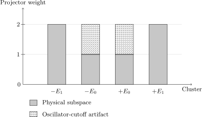
Four default energy clusters, shown as categories. Here $K=12$, $m=1$, $q=-1$, $B=0.7$, $p_z=0.4$, and $\hbar=c=1$. The energies are $E_0\approx1.077033$ and $E_1=1.6$. All four raw multiplicities are two, but the projector weights distinguish the physical lowest level from its cutoff artifact.

In the cluster CSV, physical_N0_weight is already part of physical_interior_weight. Do not add both when accounting for the total. The disjoint decomposition is the physical interior, the boundary-adjacent physical $N=K-1$ sector, and the spurious top sector. The boundary-adjacent physical block is exact for this model, but is excluded from the reported low-sector cutoff comparisons.

Cutoff, zero modes, and massive limits

The independent cutoff study constructs matrices at $K=6,10,14$ and compares fixed physical $N=0,1,2,3$ sectors. The largest energy discrepancy is about $4.44\times10^{-16}$ in the retained run. This roundoff-level agreement reflects exact invariant blocks already contained in each matrix; it is not evidence for a fitted algebraic convergence rate. A sorted eigenvalue index is a poor comparison label because its physical sector can change as the matrix grows.

At exactly $m=p_z=0$, the physical $N=0$ positive and negative branches coalesce into one two-dimensional zero space. The finite matrix also contains two artificial zero states, giving a raw cluster of dimension four. The program does not evaluate $(I\pm H/E)/2$ at $E=0$ or count the coalesced physical space twice. Very small but nonzero gaps that cannot be resolved at the declared clustering tolerance are rejected rather than relabeled as this exact apex.

The separate nonrelativistic CSV uses a fixed massive fixture, even when the configured spectral run is massless. For its scalar value $F_N=p_z^2+2|q|\hbar BN$, it compares

$$\begin{aligned} E_N-mc^2 ={}&\frac{F_N}{2m} -\frac{F_N^2}{8m^3c^2}\\ &+O(c^{-4}). \end{aligned}$$

The full $F_N^2$ is retained. Decimal arithmetic verifies the positive remainder bounds discussed in the FW notebook. For $N=0,\ldots,4$, the last measured orders approach four, ranging from approximately 3.98495 to 3.99958. These are massive fixed-field limits, not an expansion in $1/m$ at $m=0$.

Reproduce the spectrum and multiplicity audit

Download the standalone Python program. The default run used Python 3.12.14 and NumPy 2.3.5 and passed 1,748 checks, including 60 exact rational assertions across twenty parameter fixtures. Those fixtures use an unnormalized ladder basis with its factorial Gram matrix, so Hermiticity is checked in that weighted inner product.

python -m pip install numpy==2.3.5
python relativistic-landau-levels.py --output-dir landau-results

Defaults are the parameters in the figure, with physical levels through $N=4$ exported. Existing outputs are protected. Two useful fresh runs are:

python relativistic-landau-levels.py --charge 1 --cutoff 20 --output-dir landau-positive-charge
python relativistic-landau-levels.py --mass 0 --pz 0 --output-dir landau-zero-mode

Download	Contents
Raw spectrum CSV	All 48 default eigenvalues and first-order residuals
Clusters CSV	Degenerate-cluster multiplicities and invariant projector weights
Levels CSV	Analytic physical branches, seed labels, spin means, and variances
Spinors CSV	Coefficients of the normalized first-order physical modes
Cutoff CSV	Fixed low-sector comparisons across independent oscillator cutoffs
Nonrelativistic CSV	Separate massive energy expansion and decimal remainder bounds
JSON report	Checks, tolerances, parameters, environment, limitations, and hashes

The public JSON uses download paths; its numerical fields and the CSV bytes retain the executed run’s results. The cluster file contains a quoted JSON array in its final column. Use a quote-aware CSV reader, even if plotting only the earlier numeric columns.

For the figure, place the default cluster CSV beside the TikZ source and use PGFPlots 1.18:

latex notebook-landau-multiplicity.tex
dvisvgm --no-fonts notebook-landau-multiplicity.dvi

The figure selects default records for $-E_1,-E_0,+E_0,+E_1$. Select the corresponding clusters afresh if changing the output parameters or row layout.

Exercises

A trace obstruction. Explain why no finite square matrices can satisfy $[a,a^\dagger]=I$, and check that the exported finite commutator avoids the contradiction.

Solution

The trace of any finite matrix commutator vanishes by cyclicity, whereas $\operatorname{tr}I=K$. The boundary correction has trace $-K$, so $\operatorname{tr}(I-K|K-1\rangle \langle K-1|)=0$, as required.

Mix the lowest-level eigenvectors. Rotate the two columns in a nonzero lowest-energy cluster by an arbitrary $2\times2$ unitary. Which physical multiplicity diagnostic survives, and why?

Solution

The individual columns can each contain both physical and artificial components. The trace of the physical projector on the complete cluster remains one: cyclicity and $WW^\dagger=I$ remove the unitary rotation. The artificial weight likewise remains one. Raw energy multiplicity alone remains two and cannot make this distinction.

A misleading convergence study. Suppose the two lowest positive eigenvalues agree with $E_0$ for every tested $K$. What additional calculation is needed before reporting two physical states?

Solution

Resolve the cluster against the known physical and boundary sector projectors. One unit of weight belongs to the opposite-spin top artifact for every cutoff. Energy stability therefore does not imply that both states approximate physical lowest-level modes.

References

• Bjorken, James D., and Sidney D. Drell. Relativistic Quantum Mechanics. McGraw–Hill, 1964.
• Thaller, Bernd. The Dirac Equation. Springer, 1992. doi:10.1007/978-3-662-02753-0.