Klein–Gordon Wave Packets

A Klein–Gordon packet requires both an initial field and its initial time derivative. This experiment evolves both data exactly within a finite Fourier basis, compares three preparations, and measures how the periodic box and momentum cutoff affect the answer. The plotted field intensity is a shape diagnostic; the conserved Klein–Gordon pairing is a separate, signed quantity. The derivation of the modes belongs to Plane-Wave Solutions.

Required background. Plane-Wave Solutions supplies the two-data evolution; Klein–Gordon Inner Product fixes the pairing. Helpful background. Klein–Gordon to Schrödinger provides the low-momentum comparison and its error bounds.

Run the investigation. The program and retained results below support the stated experiment. Follow Running an Experiment for environment and output-directory guidance. The recorded evidence applies to its stated parameters and environment.

Two Cauchy data on a periodic Fourier grid

Use one spatial dimension, $\hbar=c=1$, mass $m>0$, and a periodic interval $[-L/2,L/2)$ with even $N$ and spacing $\Delta x=L/N$. Let $f(x)=\phi(0,x)$ and $h(x)=\partial_t\phi(0,x)$. For each retained Fourier wave number $k=2\pi n/L$, set $E_k=\sqrt{k^2+m^2}$. The implemented evolution is

$$\begin{aligned} \widehat\phi_k(t) &=\widehat f_k\cos(E_kt) +\frac{\widehat h_k}{E_k}\sin(E_kt),\\ \widehat{\partial_t\phi}_k(t) &=-E_k\widehat f_k\sin(E_kt) +\widehat h_k\cos(E_kt). \end{aligned}$$

No numerical time integrator is used. Changing the output times samples the same exact finite-mode solution. The independent frequency reconstruction uses

$$\begin{aligned} a_k&=\frac12(\widehat f_k+i\widehat h_k/E_k),\\ b_k&=\frac12(\widehat f_k-i\widehat h_k/E_k),\\ \widehat\phi_k(t)&=a_ke^{-iE_kt}+b_ke^{iE_kt}. \end{aligned}$$

Both branches retain the same spatial Fourier phase. Positive frequency means $\widehat h_k=-iE_k\widehat f_k$, not $h=0$.

NumPy’s unitary FFT is used in both directions. Its coefficients are finite box coefficients, with Parseval identity

$$\Delta x\sum_j|f_j|^2 =\Delta x\sum_k|\widehat f_k|^2.$$

They are not continuum momentum amplitudes with an unstated factor of $2\pi$ or $\Delta k$.

The adopted massive pairing gives

$$\begin{aligned} \rho&=-\frac1m\operatorname{Im}(\phi^*\partial_t\phi),\\ j&=\frac1m\operatorname{Im}(\phi^*\partial_x\phi),\\ Q&=\Delta x\sum_k\frac{E_k}{m} \bigl(|a_k|^2-|b_k|^2\bigr). \end{aligned}$$

The code compares $Q$ with $\Delta x\sum_j\rho_j$. Neither $\rho$ nor $|\phi|^2$ is asserted to be a general positive local probability density. The latter’s centroid and width describe the field shape. A real nonzero solution can have $Q=0$.

Run and inspect the three preparations

Download klein-gordon-wave-packets.py. The standalone calculation uses only NumPy and Python’s standard library and performs no network access. It is import-safe for use in a personal notebook. The retained execution used Python 3.12.14 and NumPy 2.3.5.

In a Python 3.12 virtual environment:

python -m pip install "numpy==2.3.5"
python klein-gordon-wave-packets.py --output-dir kg-run

Use a new output directory. The default report has "passed": true and 64 scientific checks. Existing output files are refused. --help describes parameters and optional destination overrides.

The default field profile is a Gaussian with center $-6$, field-intensity standard deviation $2$, and carrier momentum $0.9$. It uses $m=1$, $L=128$, $N=1024$, and five output times from $0$ through $24$. Three preparations share the grid:

Preparation	Initial derivative and interpretation
positive_frequency	The nonlocal spectral derivative $-iE_k\widehat f_k$, with $b_k=0$
independent_cauchy_data	A separately specified shifted complex Gaussian derivative; both branches are present
real_zero_derivative	A real Gaussian and $h=0$; equal positive/negative weights and zero signed charge

The initial Gaussian is normalized in the flat field norm, not rescaled to unit KG charge. Accordingly the default positive-frequency charge is about $1.35857313$, not one. This difference is an intentional normalization check.

Packet motion and reproducible outputs

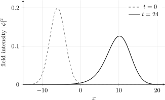
Default positive-frequency field intensity at $t=0$ and $t=24$. The centroid moves from $-6$ to $9.59716$, and the shape standard deviation grows from $2$ to $3.34526$. These are moments of $|\phi|^2$, not moments of a proposed KG position probability. The displayed window lies well inside the periodic box.

The full retained outputs are:

Download	Contents
Summary and checks	Versions, parameters, program/CSV hashes, tolerances, and all checks
Profiles	Real/imaginary field and time derivative, intensity, signed charge density, and current
Diagnostics	Frequency weights, charge, energy, field-shape moments, edge and cutoff fractions
Refinement studies	Independent box, cutoff, and derivative-residual experiments
Nonrelativistic comparison	Rest-phase-removed errors and weighted momentum bounds

Published report paths are normalized to the download locations; numerical results and CSV bytes are unchanged. The fixed verification fixtures in the report are distinct from user-selected profile parameters. Passing those fixtures does not certify an arbitrary new packet or box.

To reproduce the figure, place its TikZ/PGFPlots source beside the retained profiles.csv and run:

latex notebook-klein-gordon-packet.tex
dvisvgm --no-fonts notebook-klein-gordon-packet.dvi

The source also resolves the data from the repository root. Its row selections are explicitly tied to the default $1024$-point, five-time output. Changing --points or --time-samples requires updating those selections; do not plot a different preparation under the old caption.

Separate box, cutoff, and diagnostic derivative errors

At fixed $L=128$, increasing $N$ changes the largest retained wave number. The cutoff study compares both Cauchy data on common spatial samples against a finer reference in the same box. At fixed $\Delta x=0.125$, increasing $L$ instead moves the periodic images away without increasing the cutoff. That study compares the same physical window $-12\le x\le12$.

Representative retained results are:

Study	Result
Fixed box, $N=64$	Relative Cauchy-data error $0.1022$
Fixed box, $N=128$	Error $8.35\times10^{-10}$
Fixed box, $N\ge256$	Agreement with the finer reference at about $4.5\times10^{-15}$
Fixed spacing, $L=32$	Common-window error $0.01816$ and about $16\%$ intensity in the outer edge zones
Fixed spacing, $L\ge64$	Common-window agreement with the $L=512$ reference at about $2.4\times10^{-15}$

Small finite-reference differences are numerical evidence for these fixtures, not a universal continuum convergence proof. Inspect the edge fractions of the field, time derivative, and energy, as well as the sector-weight and energy fractions near the Fourier cutoff. A narrow high-momentum packet can defeat a grid that resolves a broad slow packet.

The independent time-difference check approximates derivatives of the exact solution. Its KG residual decreases from $1.16\times10^{-3}$ at diagnostic $\Delta t=0.08$ to $1.81\times10^{-5}$ at $0.01$, consistent with a second-order difference formula. This is not an integration-step convergence result.

Check the nonrelativistic approximation with its tail

A separate low-momentum fixture uses $m=2$, mean momentum $0.2$, and momentum standard deviation $0.1$. After removing the rest phase, the exact frequency is

$$E_k-m=\frac{k^2}{E_k+m}.$$

The rationalized expression avoids a small difference of large energies. Compare it with $k^2/(2m)$ and $k^2/(2m)-k^4/(8m^3)$. For normalized spectral weights, the relative field-norm errors obey the moment bounds

$$\begin{aligned} \epsilon_{\rm Sch}(t) &\le\frac{|t|}{8m^3}\sqrt{\langle k^8\rangle},\\ \epsilon_{\rm fourth}(t) &\le\frac{|t|}{16m^5}\sqrt{\langle k^{12}\rangle}. \end{aligned}$$

The derivation belongs to Klein–Gordon to Schrödinger. The numerical weights include the retained Gaussian tail; no false hard momentum cutoff is assigned to the Gaussian.

At $t=40$, the Schrödinger relative error is $0.00519071$, below the quartic-moment bound $0.00530072$. The fourth-order error is $0.000117730$, below the sixth-moment bound $0.000121794$. The report also retains a tighter bound formed from the exact phase-energy difference. These results concern this separate low-momentum fixture, not the $0.9$-momentum packet in the figure.

Modification exercises

A field at rest in time is not positive frequency. Replace the positive-frequency preparation by $h=0$ while keeping nonzero $f$. What must the sector diagnostic report?

Solution

$a_k=b_k=\widehat f_k/2$. Their positive and negative weights are equal, so $Q=0$, although the field and its positive energy functional need not vanish. If $f$ is real, the evolved solution remains real.

A misleading refinement. Increase $L$ while keeping $N$ fixed. Why is this not a clean box-size test?

Solution

$\Delta x=L/N$ increases, so the Nyquist wave number $\pi/\Delta x$ decreases. The periodic images move outward while the momentum resolution at high wave number worsens. A box test should keep $\Delta x$ fixed, and a separate cutoff test should keep $L$ fixed.

Change the mass without changing the claim. Run a smaller positive --mass at the same profile momentum. Which comparison needs renewed justification?

Solution

The ratio of characteristic momentum to mass grows, weakening a nonrelativistic approximation. Inspect the new profile’s edge/cutoff diagnostics and, for a new NR comparison, recompute its own spectral weights and error bounds. The fixed low-momentum verification fixture does not change automatically with the profile. Setting $m=0$ is rejected because this notebook’s pairing divides by $m$.

References

• Bjorken, James D., and Sidney D. Drell. Relativistic Quantum Mechanics. McGraw–Hill (1964). Scalar modes and relativistic currents.
• Greiner, Walter. Relativistic Quantum Mechanics: Wave Equations. 3rd ed., Springer (2000). doi:10.1007/978-3-662-04275-5. Frequency branches and scalar wave mechanics.