Born Approximation Numerical Test

A smooth Born curve can look plausible long after first-order scattering has stopped being quantitative. This notebook asks a sharper question: for which potential strengths and incident momenta does the first Born total cross section agree with a separately converged partial-wave calculation to a stated tolerance?

The test potential is a repulsive three-dimensional Gaussian. Repulsion deliberately removes bound-state and resonance poles from the comparison, so the observed loss of accuracy is a clean failure of weak repeated-scattering control rather than a hidden threshold state. A NumPy-only program integrates the radial Schrödinger equation, extracts phase shifts, reconstructs elastic observables, sweeps coupling and momentum, and writes every retained data table.

The principal result is observable-specific. At fixed dimensionless momentum $\kappa=1.5$, the Born total cross section is accurate to $2.12\%$ at coupling $\nu=0.25$, but its error rises to $11.4\%$ at $\nu=1$ and $93.4\%$ at $\nu=4$. Increasing momentum improves this particular short-range problem: at $\nu=4$, the error falls from $372\%$ at $\kappa=0.5$ to $5.98\%$ at $\kappa=4$.

Run the investigation. The program and retained results below support the stated experiment. Follow Running an Experiment for environment and output-directory guidance. The recorded evidence applies to its stated parameters and environment.

Canonical Boundaries

This page owns one reproducible numerical experiment, not the general scattering formalism.

Object	Canonical home	Role here
Fourier-transform derivation of $f_{\mathrm B}$	First Born Approximation	analytic target
general validity criteria and pole warnings	Validity of the Born Approximation	interpretation of the sweep
Gaussian transform and Born cross section	Gaussian Potential in the Born Approximation	closed-form benchmark
generic phase extraction workflow	Phase Shift Extraction	numerical method specialized here
partial-wave amplitude and unitarity	Partial-Wave Expansion	reconstruction and structural checks

The new content is the coupling-momentum regime map, its numerical error ledger, and the downloadable implementation and data.

Physical Problem

Consider elastic scattering with reduced mass $\mu$ from

$$V(r) = V_0e^{-r^2/a^2}, \qquad V_0>0.$$

The stationary Schrödinger equation is

$$\left[ -\frac{\hbar^2}{2\mu}\nabla^2 +V(r) \right] \psi = \frac{\hbar^2k^2}{2\mu}\psi.$$

Use the range $a$ as the unit of length and define

$$\rho=\frac{r}{a}, \qquad \kappa=ka, \qquad \nu=\frac{2\mu V_0a^2}{\hbar^2}.$$

The dimensionless radial equation for the reduced wavefunction is

$$\frac{d^2u_\ell}{d\rho^2} + \left[ \kappa^2 -\nu e^{-\rho^2} -\frac{\ell(\ell+1)}{\rho^2} \right] u_\ell =0.$$

Only two physical parameters remain:

• $\kappa$ compares the potential range with the incident wavelength;
• $\nu$ compares the potential strength with the localization energy $\hbar^2/(2\mu a^2)$.

For this shape, the low-energy weak-coupling scale is of order $\nu$, while the high-energy accumulated-phase scale is of order $\nu/\kappa$. Those are scaling guides, not universal error bars.

Why use a repulsive potential?

An attractive Gaussian can develop a near-threshold bound state. Its scattering length then becomes large, and a Born failure may be dominated by a nonperturbative pole. That is important physics, but it would mix two questions. The repulsive model has no bound states, so this notebook isolates ordinary distortion and repeated scattering.

The conclusion must not be transferred blindly to attraction. A second experiment with $V_0<0$ should explicitly monitor the scattering length and bound-state thresholds.

Analytic Target

With the amplitude convention

$$\psi_{\mathbf k}^{(+)}(\mathbf r) \sim e^{i\mathbf k\cdot\mathbf r} + f(\theta)\frac{e^{ikr}}{r},$$

the Gaussian first Born amplitude becomes

$$\frac{f_{\mathrm B}(\theta)}{a} = -\frac{\sqrt\pi}{4}\nu \exp\left[ -\kappa^2\sin^2\frac{\theta}{2} \right].$$

Therefore

$$\frac{1}{a^2} \frac{d\sigma_{\mathrm B}}{d\Omega} = \frac{\pi\nu^2}{16} \exp\left[ -2\kappa^2\sin^2\frac{\theta}{2} \right],$$

and angular integration gives

$$\frac{\sigma_{\mathrm B}}{a^2} = \frac{\pi^2\nu^2}{8\kappa^2} \left( 1-e^{-2\kappa^2} \right).$$

The code evaluates the last expression with expm1 to avoid subtractive loss when $\kappa$ is small.

For a coupling sweep $V\to\nu V_*$, the exact amplitude has the weak-coupling form

$$f(\nu) = \nu f^{(1)} + \nu^2 f^{(2)} + O(\nu^3).$$

Away from an amplitude zero, the cross section consequently has the structure

$$\sigma(\nu) = \nu^2\sigma^{(2)} + \nu^3\sigma^{(3)} + O(\nu^4).$$

Thus the relative first Born cross-section error should initially scale as $O(\nu)$, even though the Born cross section itself is $O(\nu^2)$.

Numerical Benchmark

The comparison labelled “numerical” below is a converged solution of the same single-channel central-potential model. It is not an analytic exact solution and does not remove model error.

Numerov propagation

Write

$$u_\ell''(\rho) +Q_\ell(\rho)u_\ell(\rho) =0,$$

with

$$Q_\ell(\rho) = \kappa^2 -\nu e^{-\rho^2} -\frac{\ell(\ell+1)}{\rho^2}.$$

On a uniform grid $\rho_n=nh$, the implemented Numerov step is organized as

$$\begin{aligned} N_n &= 2\left(1-\frac{5h^2Q_n}{12}\right)u_n \\ &\quad- \left(1+\frac{h^2Q_{n-1}}{12}\right)u_{n-1}, \\ D_n &= 1+\frac{h^2Q_{n+1}}{12}, \\ u_{n+1} &= \frac{N_n}{D_n}. \end{aligned}$$

The regular origin solution is seeded with the first Frobenius correction,

$$u_\ell(\rho) \propto \rho^{\ell+1} \left[ 1+ \frac{\nu-\kappa^2}{4\ell+6}\rho^2 +O(\rho^4) \right].$$

This correction makes coarse-grid convergence less sensitive to the arbitrary first two points. The overall normalization is irrelevant to phase matching.

Asymptotic matching

At a radius $\rho_m$ where the Gaussian tail is negligible, write

$$u_\ell(\rho) = C_\ell \left[ \widehat j_\ell(\kappa\rho)\cos\delta_\ell - \widehat n_\ell(\kappa\rho)\sin\delta_\ell \right],$$

where

$$\widehat j_\ell(z)=zj_\ell(z), \qquad \widehat n_\ell(z)=zn_\ell(z).$$

The five-point derivative is

$$\begin{aligned} u_m' &= \frac{u_{m-2}-8u_{m-1}}{12h} \\ &\quad+ \frac{8u_{m+1}-u_{m+2}}{12h} +O(h^4). \end{aligned}$$

Let $J=\widehat j_\ell(z)$, $N=\widehat n_\ell(z)$, and $z=\kappa\rho_m$, with primes denoting $z$ derivatives. The phase is computed without dividing by $u_m$:

$$\begin{aligned} A_\ell &= \kappa J'u_m-Ju_m', \\ B_\ell &= \kappa N'u_m-Nu_m', \\ \delta_\ell &= \operatorname{atan2}(A_\ell,B_\ell) \pmod{\pi}. \end{aligned}$$

Using both $u_m$ and $u_m'$ avoids a singular logarithmic derivative when the match point happens to lie near a radial node.

Stable special functions

The regular Riccati–Bessel sequence is the minimal solution when $\ell$ exceeds $z$. Upward recurrence can then amplify roundoff. The program uses Miller downward recurrence for $\widehat j_\ell$ and stable upward recurrence for the dominant $\widehat n_\ell$ sequence. It checks the Wronskian

$$J N'-J'N=1$$

over every order and matching argument needed by the production sweep. The maximum retained residual is $1.33\times10^{-15}$.

Reconstructing observables

The partial-wave amplitude is

$$\begin{aligned} \frac{f_{\mathrm{num}}(\theta)}{a} &= \frac{1}{\kappa} \sum_{\ell=0}^{\ell_{\max}} \mathcal A_\ell(\theta), \\ \mathcal A_\ell(\theta) &= (2\ell+1)e^{i\delta_\ell}\sin\delta_\ell \\ &\quad\times P_\ell(\cos\theta). \end{aligned}$$

The integrated elastic cross section is evaluated directly from the phases:

$$\frac{\sigma_{\mathrm{num}}}{a^2} = \frac{4\pi}{\kappa^2} \sum_{\ell=0}^{\ell_{\max}} (2\ell+1)\sin^2\delta_\ell.$$

The primary discrepancy is

$$\epsilon_\sigma = \frac{ \left| \sigma_{\mathrm B}-\sigma_{\mathrm{num}} \right| }{ \sigma_{\mathrm{num}} }.$$

An integrated positive observable avoids division by a Born diffraction zero. It can still hide angular compensation, so the angular distributions are retained separately.

Production Parameters

Control	Production value	Sweep or check
coupling	$0.02\le\nu\le8$	logarithmic grid plus quoted anchors
momentum	$\kappa=0.5,1,2,4$	independent curves
radial step	$h/a=0.0025$	$0.04$ down to $0.00125$
matching radius	$\rho_m=10$	$4,5,6,8,10,12$
partial-wave cutoff	$\ell_{\max}=16$	$2$ through $18$
angular samples	$181$	$0^\circ$ through $180^\circ$
arithmetic	IEEE 754 binary64	deterministic, no random seed

At the shortest production wavelength, $\kappa=4$, the grid has about $628$ points per radial wavelength. This is deliberately much finer than necessary; the convergence sweep, rather than that count alone, establishes adequacy.

Coupling-Momentum Regime Map

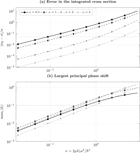
Panel (a) compares the analytic Born total cross section with the converged partial-wave result. The horizontal guide is $5\%$. Panel (b) shows $\max_\ell|\delta_\ell|$ on the principal branch, with a $0.1$ guide. Higher momentum improves this smooth short-range model, but neither guide is a universal validity boundary.

Three features are visible.

1. The weak-coupling error is linear in $\nu$. At $\kappa=1.5$, doubling $\nu$ from $0.05$ to $0.1$ changes $\epsilon_\sigma$ from $0.386\%$ to $0.792\%$, consistent with the expected $O(\nu)$ relative error.
2. Increasing momentum helps. At $\nu=4$, the errors for $\kappa=0.5,1,2,4$ are respectively $372\%$, $210\%$, $40.9\%$, and $5.98\%$.
3. Small phase shifts are useful but not a complete error bar. At $\kappa=4$ and $\nu=1$, the largest principal phase is $0.112$, while the total-cross-section error is only $0.742\%$. Cancellation and observable weighting matter.

For the intermediate momentum $\kappa=1.5$, the retained values are:

| $\nu$ | $\sigma_{\mathrm{num}}/a^2$ | $\sigma_{\mathrm B}/a^2$ | $\epsilon_\sigma$ | $\max|\delta_\ell|$ | |---:|---:|---:|---:|---:| | $0.05$ | $0.00135033$ | $0.00135555$ | $0.386\%$ | $0.0132$ | | $0.25$ | $0.0331844$ | $0.0338888$ | $2.12\%$ | $0.0656$ | | $0.5$ | $0.129432$ | $0.135555$ | $4.73\%$ | $0.130$ | | $1$ | $0.486537$ | $0.542220$ | $11.4\%$ | $0.255$ | | $2$ | $1.65613$ | $2.16888$ | $31.0\%$ | $0.480$ | | $4$ | $4.48663$ | $8.67552$ | $93.4\%$ | $0.831$ | | $8$ | $8.74793$ | $34.7021$ | $297\%$ | $1.245$ |

The Born cross section grows as $\nu^2$ for all couplings because the approximation contains no saturation mechanism. The exact partial waves obey unitarity channel by channel, so their growth is constrained. That structural difference becomes dominant at strong coupling.

Angular Structure and Grid Convergence

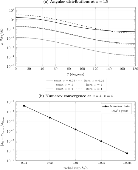
Panel (a) compares converged partial-wave curves (solid) with first Born curves (dashed) at $\kappa=1.5$. Weak coupling preserves both scale and shape; at $\nu=4$, the integrated Born excess is large even though the curves can cross at some angles. Panel (b) uses the hardest momentum in the regime sweep, $\kappa=4$, at $\nu=4$ and shows fourth-order convergence toward the $h/a=0.00125$ reference.

The angular comparison explains why a total cross section cannot be the only reported observable. At $\nu=4$, the Born prediction is much too large in the forward region, but the backward curves are closer and can cross. An integrated discrepancy is a weighted summary, not a uniform angular error bound.

The lower panel also separates numerical and physical error. For $\kappa=4$ and $\nu=4$,

$$\epsilon_\sigma^{\mathrm{Born}} = 5.98\times10^{-2},$$

while the production-grid change relative to the finest run is

$$\epsilon_h = 5.37\times10^{-9}.$$

The measured Born discrepancy is therefore not a radial-grid artifact.

Convergence Ledger

Radial step

The most oscillatory production point, $\kappa=4$, is tested at the strong coupling $\nu=4$ with $\ell_{\max}=16$.

$h/a$	$\sigma_h/a^2$	relative difference from $h/a=0.00125$
$0.04$	$1.1636865465$	$3.83\times10^{-4}$
$0.02$	$1.1641044824$	$2.37\times10^{-5}$
$0.01$	$1.1641303884$	$1.48\times10^{-6}$
$0.005$	$1.1641320010$	$9.18\times10^{-8}$
$0.0025$	$1.1641321016$	$5.37\times10^{-9}$
$0.00125$	$1.1641321078$	reference

Successive triples give observed orders near $4.00$. The formal Numerov propagation has higher local order, but the five-point derivative and phase extraction make fourth-order behavior the relevant end-to-end expectation for this implementation.

Partial-wave cutoff

At the same physical point:

$\ell_{\max}$	relative cross-section difference from $\ell_{\max}=18$	last retained partial-wave fraction
$4$	$3.97\times10^{-2}$	$8.41\times10^{-2}$
$6$	$2.29\times10^{-3}$	$8.30\times10^{-3}$
$8$	$6.10\times10^{-5}$	$3.49\times10^{-4}$
$10$	$8.26\times10^{-7}$	$6.86\times10^{-6}$
$12$	$6.22\times10^{-9}$	$7.06\times10^{-8}$
$16$	$7.78\times10^{-14}$	$1.48\times10^{-12}$

The last-wave fraction is a useful stopping diagnostic, but agreement under an explicit cutoff sweep is stronger evidence. A tiny final term can occasionally follow an earlier cancellation.

Matching radius

The Gaussian tail is already small at $\rho=4$ and negligible at the production match point.

$\rho_m$	$\nu e^{-\rho_m^2}$	relative difference from $\rho_m=12$
$4$	$4.50\times10^{-7}$	$5.75\times10^{-8}$
$5$	$5.56\times10^{-11}$	$4.99\times10^{-9}$
$6$	$9.28\times10^{-16}$	$4.32\times10^{-9}$
$8$	$6.42\times10^{-28}$	$2.91\times10^{-9}$
$10$	$1.49\times10^{-43}$	$1.46\times10^{-9}$
$12$	$1.16\times10^{-62}$	reference

Beyond $\rho_m=5$, the residual variation is controlled by the finite radial step and phase extraction rather than by a physical potential tail.

Independent Checks

Free-potential limit

Setting $\nu=0$ must give

$$\delta_\ell=0$$

for every retained partial wave. The maximum error over the low- and intermediate-momentum tests is

$$\max_\ell|\delta_\ell^{(\nu=0)}| = 2.88\times10^{-10}.$$

This test exercises the origin seed, Numerov recurrence, derivative, Bessel sequences, match convention, and branch wrapping together.

Weak-coupling limit

At $\kappa=1.5$ and $\nu=0.01$, the numerical and Born total cross sections differ by

$$7.57\times10^{-4}$$

relatively. Repeating the sweep rather than checking only one weak point confirms the expected linear decrease of the relative error.

Elastic unitarity

The reconstructed amplitude and partial-wave cross section obey

$$\operatorname{Im} \frac{f_{\mathrm{num}}(0)}{a} = \frac{\kappa}{4\pi} \frac{\sigma_{\mathrm{num}}}{a^2}.$$

The production residual is $1.50\times10^{-16}$. This is a structural check of amplitude assembly because both sides use the same phases. It does not independently validate the radial differential-equation solution.

The real first Born amplitude does not satisfy the exact optical theorem by itself. That is not a contradiction: $|f^{(1)}|^2$ is second order in the coupling, and the matching imaginary forward term first appears in $f^{(2)}$. Optical Theorem and Unitarity own that order-by-order statement.

Error Budget at the Hardest Grid Point

For $\kappa=4$ and $\nu=4$:

Source	Retained estimate	Interpretation
Born truncation	$5.98\times10^{-2}$	physical approximation error
radial step	$5.37\times10^{-9}$	production versus refined grid
matching radius	$1.46\times10^{-9}$	$\rho_m=10$ versus $12$
partial-wave cutoff	$7.78\times10^{-14}$	$\ell_{\max}=16$ versus $18$
Bessel Wronskian	$1.33\times10^{-15}$	special-function consistency
optical-theorem assembly	$1.50\times10^{-16}$	partial-wave reconstruction

The numerical benchmark is resolved well below the approximation error. Quoting additional digits in the Born answer would not improve its physical accuracy.

What the Regime Map Does and Does Not Show

The data support the qualitative high-energy phase estimate $\nu/\kappa$: for fixed $\nu$, increasing $\kappa$ generally improves the first Born total cross section. They do not establish a universal boundary such as

$$\frac{\nu}{\kappa}<c$$

for a fixed constant $c$. The error also depends on potential shape, angular region, observable, and tolerance.

Likewise, the condition

$$\max_\ell|\delta_\ell|\ll1$$

is a channel-resolved warning sign, not an exact error estimator. Some observables weight many phases with cancellations; others are dominated by one channel or by a diffraction minimum. The figure therefore plots both the physical error and the phase diagnostic instead of using one as a proxy for the other.

Reproduce the Calculation

Run the downloaded program from the folder where you saved it:

python born-approximation-numerical-test.py --output-dir results

NumPy is the only required package. The optional —plot flag uses Matplotlib to make quick-look PNGs; the documentation figures are rendered from the retained CSV data with the linked TeX sources.

Artifact	Contents
Python program	solver, sweeps, checks, and data export
strength summary	quoted $\kappa=1.5$ table
regime curves	coupling and momentum sweep
angular distributions	numerical and Born curves at three strengths
radial-step convergence	fourth-order refinement data
partial-wave convergence	cutoff and tail fractions
matching-radius convergence	tail and match stability
regime figure source	pgfplots source
angular/convergence figure source	pgfplots source

Retained run metadata

Item	Value
run date	2026-07-16
Python	3.12.13
NumPy	2.3.5
arithmetic	binary64
random sampling	none
wall time on retained machine	$8.38\ \mathrm{s}$
code license	MIT
figure data	unfiltered CSV output

Runtime is hardware-dependent and is not a validation target. Reproduction should compare data values and embedded checks, not elapsed time.

Known Failure Modes

• Matching inside the potential tail: free Riccati–Bessel matching is invalid until $V(\rho_m)$ is negligible at the requested tolerance.
• Insufficient angular-momentum cutoff: the needed cutoff grows with $\kappa$ and interaction range. A fixed $\ell_{\max}$ is not portable to a new regime.
• Unstable special-function recurrence: upward recurrence for the regular spherical Bessel sequence can fail when $\ell\gtrsim z$.
• Phase branch jumps: $\delta_\ell$ is defined modulo $\pi$ for the elastic observables used here. Continuous energy sweeps require explicit unwrapping.
• Relative errors near angular zeros: a tiny denominator can make a pointwise relative error meaningless. Use absolute or binned errors there.
• Long-range interactions: the free short-range matching and ordinary Born transform do not handle an unscreened Coulomb tail.
• Singular potentials: origin seeding and higher Born terms may require regularization or a different propagator.
• Attractive near-threshold physics: a shallow state can invalidate first order far earlier than the repulsive regime map suggests.
• High momentum without refinement: larger $\kappa$ needs a smaller radial step and generally a larger partial-wave cutoff, even though the physical Born approximation may improve.
• Treating total agreement as angular agreement: cancellations can make an integrated observable look better than its differential distribution.

For stiff, multichannel, or very long propagation problems, a renormalized Numerov or log-derivative propagator can be more robust than the direct scalar implementation used here.

Further Investigations

Natural extensions should change one scientific question at a time.

1. Repeat the sweep for an attractive Gaussian and locate the first scattering-length pole.
2. Compute the second Born amplitude and test whether it reduces the weak-coupling residual with the expected order.
3. Compare first Born with an eikonal approximation at large $\kappa$ and moderate $\nu$.
4. Map differential rather than total error over $(\theta,\nu,\kappa)$ using finite angular bins.
5. Replace Numerov matching with a variable-phase or log-derivative method and compare independent numerical errors.

Exercises

Integrate the Born angular distribution

Starting from

$$\frac{1}{a^2} \frac{d\sigma_{\mathrm B}}{d\Omega} = \frac{\pi\nu^2}{16} e^{-\kappa^2(1-\cos\theta)},$$

derive the total Born cross section used by the program.

Solution

Set $x=\cos\theta$ and use $d\Omega=2\pi\,dx$:

$$\begin{aligned} \frac{\sigma_{\mathrm B}}{a^2} &= \frac{\pi^2\nu^2}{8} \int_{-1}^{1} dx\, e^{-\kappa^2(1-x)} \\ &= \frac{\pi^2\nu^2}{8\kappa^2} \left( 1-e^{-2\kappa^2} \right). \end{aligned}$$

As $\kappa\to0$, the ratio tends to $2$, giving $\sigma_{\mathrm B}/a^2\to\pi^2\nu^2/4$.

Explain the linear relative error

Suppose

$$f(\nu)=\nu f_1+\nu^2f_2+O(\nu^3).$$

Show why the relative error of the first Born cross section is generically $O(\nu)$ rather than $O(\nu^2)$.

Solution

Squaring the amplitude gives

$$|f|^2 = \nu^2|f_1|^2 + 2\nu^3 \operatorname{Re}(f_1^*f_2) +O(\nu^4).$$

The absolute cross-section correction is $O(\nu^3)$, while the leading cross section is $O(\nu^2)$. Their ratio is therefore $O(\nu)$. At an amplitude zero the leading denominator vanishes, so this argument must be replaced by an absolute or binned comparison.

Estimate the observed Numerov order

Use the cross sections at $h/a=0.04$, $0.02$, and $0.01$ to estimate

$$p_{\mathrm{obs}} = \frac{ \log \left| \dfrac{\sigma_{0.04}-\sigma_{0.02}} {\sigma_{0.02}-\sigma_{0.01}} \right| }{\log2}.$$

Solution

The successive differences are approximately

$$\begin{aligned} |\sigma_{0.04}-\sigma_{0.02}| &=4.17936\times10^{-4}, \\ |\sigma_{0.02}-\sigma_{0.01}| &=2.59061\times10^{-5}. \end{aligned}$$

Their ratio is about $16.13$, so

$$p_{\mathrm{obs}} = \frac{\log16.13}{\log2} \approx4.01.$$

This agrees with the fourth-order end-to-end behavior expected after including derivative and matching error.

Check the perturbative trend

At $\kappa=1.5$, the cross-section errors are $0.386\%$ at $\nu=0.05$ and $0.792\%$ at $\nu=0.1$. What exponent $p$ is suggested by $\epsilon_\sigma\propto\nu^p$?

Solution

The two-point estimate is

$$p = \frac{ \log(0.00792/0.00386) }{ \log(0.1/0.05) } \approx1.04.$$

This is consistent with the generic first-order relative-error prediction $p=1$. Two points do not establish an asymptotic law by themselves; the full weak-coupling sweep supplies the stronger check.

Interpret high-energy improvement

At fixed $\nu=4$, why can the Born total cross section improve strongly as $\kappa$ rises even though $\nu$ itself is not small?

Solution

For a smooth localized potential, rapid phase oscillation suppresses coherent repeated scattering. A straight-path phase estimate scales as $\nu/\kappa$, so increasing $\kappa$ can reduce distortion even at fixed strength. This is not automatic for hard cores, long-range tails, thresholds, or a specially tuned resonance, and the achieved error remains observable-dependent.

Predict the attractive-potential warning

What extra diagnostic is essential before repeating the same plot for $V_0<0$ at low momentum?

Solution

One must track the $s$-wave scattering length and the appearance of bound or virtual states near threshold. As a state approaches zero energy, the scattering length can diverge and the amplitude is controlled by a pole rather than by the small volume integral appearing in first Born theory. A coupling sweep should therefore include bound-state counting or an equivalent pole diagnostic, not only phase magnitudes and numerical convergence.

Cross-Links

• Computational Notebooks
• First Born Approximation
• Validity of the Born Approximation
• Gaussian Potential in the Born Approximation
• Phase Shift Extraction
• Partial-Wave Expansion
• Phase Shifts
• Differential and Total Cross Sections
• Optical Theorem
• Convergence Tests
• Finite-Difference Methods
• Bessel Functions

References

• M. Born, “Quantenmechanik der Stoßvorgänge,” Zeitschrift für Physik 38, 803–827 (1926), doi:10.1007/BF01397184.
• J. R. Taylor, Scattering Theory: The Quantum Theory of Nonrelativistic Collisions, Dover, 2006, Chapters 3, 9, and 11.
• R. G. Newton, Scattering Theory of Waves and Particles, 2nd ed., Dover, 2002, Chapters 11 and 12.
• C. J. Joachain, Quantum Collision Theory, 3rd ed., North-Holland, 1983, Chapters 6 and 7.
• J. M. Thijssen, Computational Physics, 2nd ed., Cambridge University Press, 2007, section on Numerov integration and radial scattering.
• B. R. Johnson, “The multichannel log-derivative method for scattering calculations,” Journal of Computational Physics 13, 445–449 (1973), doi:10.1016/0021-9991(73)90049-1.
• NIST Digital Library of Mathematical Functions, Spherical Bessel Functions and Recurrence Relations and Derivatives, accessed 2026-07-16.