Unitarity

Unitarity is conservation of total probability expressed as a constraint on scattering amplitudes. It does more than provide a final consistency check. It fixes imaginary parts, correlates different channels, confines partial-wave amplitudes to a disk, and sets energy-dependent bounds on cross sections.

The central operator statement is

$$S^\dagger S = SS^\dagger = I.$$

The identity applies to the complete scattering space with correctly normalized asymptotic channels. It does not require every elastic matrix element to have unit magnitude. If an inelastic channel is open, an elastic element may have magnitude below one while the full multichannel matrix remains exactly unitary.

Unitarity and Conservation of Probability owns the general finite-time quantum principle. S-Matrix constructs the nonrelativistic scattering operator from wave operators, and T-Matrix fixes its normalization-specific transition operator. This page is the canonical home for the constraints of scattering unitarity. Optical Theorem owns the forward-amplitude cross-section identity derived from them.

Why the Scattering Matrix Is Unitary

A closed system with self-adjoint Hamiltonian $H$ evolves unitarily. Scattering theory compares that exact evolution in the remote past and future with chosen asymptotic channel dynamics generated by $H_0$.

The Møller wave operators map free asymptotic data into the interacting scattering subspace:

$$\Omega^{(\pm)} = \operatorname*{s-lim}_{t\to\mp\infty} e^{iHt/\hbar} e^{-iH_0t/\hbar}.$$

The scattering operator is

$$S = \Omega^{(-)\dagger} \Omega^{(+)}.$$

When the wave operators exist, are isometric on the free scattering space, and are asymptotically complete, this construction gives a unitary $S$. The detailed proof and the role of the absolutely continuous subspace belong at S-Matrix.

These assumptions matter. For an unscreened long-range interaction, the reference dynamics may need to include the long-range phase. For a non-Hermitian optical potential, the reduced one-channel description is intentionally not unitary. For an incomplete channel basis, the represented matrix can lose flux into states that were left out.

Unitarity is therefore both a theorem and a diagnostic:

• it is a theorem for a self-adjoint complete scattering problem with appropriate asymptotic dynamics;
• it is a diagnostic of omitted channels, normalization errors, invalid approximations, and unconverged numerics in a practical calculation.

Energy Shell and Channel Basis

Time-translation invariance implies that $S$ commutes with the free Hamiltonian on the asymptotic space:

$$[S,H_0]=0.$$

The scattering operator is consequently block diagonal in the conserved energy. On each energy shell,

$$S^\dagger(E)S(E) = I_E.$$

Choose a flux-normalized basis of open channels $\lvert E,\alpha\rangle$. Channel labels can include particle species, internal states, spin, orbital angular momentum, and every other conserved label needed to specify asymptotic motion. Then

$$\sum_\gamma S_{\gamma\alpha}^*(E) S_{\gamma\beta}(E) = \delta_{\alpha\beta}.$$

The diagonal case is

$$\sum_\gamma \left| S_{\gamma\alpha}(E) \right|^2 = 1.$$

This is a column-sum rule: every possible open final channel $\gamma$ must be included for a fixed incoming channel $\alpha$. In a continuum, the sum also contains the appropriate momentum, angular, or many-body phase-space integrals.

Closed channels do not carry asymptotic flux and do not appear as final states in this sum. They can still modify the open-channel amplitudes virtually. When a threshold opens, the newly propagating channel joins the unitarity sum and generally changes the analytic behavior of every coupled amplitude.

Why flux normalization matters

If channel wavefunctions are normalized to equal amplitude rather than equal flux, different channel velocities introduce weights. The invariant statement is a balance of probability current. In a basis with explicit velocities,

$$\sum_\gamma v_\gamma \left| A_{\gamma\alpha} \right|^2 = v_\alpha,$$

schematically. Rescaling to unit-flux channel states absorbs the velocity factors and restores the simple matrix equation $S^\dagger S=I$.

Plane-wave matrix elements contain delta functions and are not probabilities by themselves. The channel sum rule should be interpreted using normalized wave packets or after the overall conservation delta functions have been removed consistently.

Consequences for Transition Amplitudes

To expose the algebra without committing to one continuum normalization, write the energy-shell operator schematically as

$$S=I+i\mathcal T.$$

Then

$$\begin{aligned} S^\dagger S &= \left( I-i\mathcal T^\dagger \right) \left( I+i\mathcal T \right) \\ &= I + i \left( \mathcal T-\mathcal T^\dagger \right) + \mathcal T^\dagger\mathcal T. \end{aligned}$$

Unitarity gives the master relation

$$i \left( \mathcal T^\dagger-\mathcal T \right) = \mathcal T^\dagger\mathcal T.$$

Taking a diagonal matrix element in an incoming state $\lvert i\rangle$ and inserting a complete set of final states gives

$$2\, \operatorname{Im} \mathcal T_{ii} = \sum_n \left| \mathcal T_{ni} \right|^2.$$

For continuous final states, this becomes a phase-space integral. The imaginary part of a forward amplitude is therefore not an optional damping term: it is required once probability can flow into on-shell final states.

The normalization-specific nonrelativistic identity

With delta-normalized wave-number states, the transition operator used in this chapter satisfies

$$\begin{aligned} T^{(+)}(E) - T^{(-)}(E) ={}& - 2\pi i \\ &\times T^{(-)}(E) \\ &\times \delta(E-H_0) \\ &\times T^{(+)}(E). \end{aligned}$$

For a self-adjoint interaction,

$$T^{(-)}(E) = T^{(+)}(E)^\dagger.$$

The diagonal relation is

$$\begin{aligned} \operatorname{Im} \langle i\lvert T^{(+)}\rvert i\rangle ={}& -\pi \sum_n \langle i\lvert T^{(-)}\rvert n\rangle \\ &\times \delta(E-E_n) \langle n\lvert T^{(+)}\rvert i\rangle. \end{aligned}$$

The sign differs from the schematic $\mathcal T$ convention because this chapter uses

$$S = I - 2\pi i\, \delta(E_f-E_i)T.$$

The nonrelativistic amplitude $f$ is proportional to $-T$ in the same convention, giving the positive forward imaginary part required by the optical theorem. Mixing these definitions without their delta functions and normalization factors is a common source of false sign contradictions.

Partial-Wave Unitarity

For spinless scattering from a short-range central potential, write

$$f(\theta) = \frac{1}{k} \sum_{\ell=0}^{\infty} (2\ell+1) a_\ell P_\ell(\cos\theta),$$

where

$$a_\ell = \frac{S_\ell-1}{2i}.$$

If the scattering is purely elastic in partial wave $\ell$, no flux can leave that channel:

$$\lvert S_\ell\rvert=1.$$

Every complex number of unit magnitude can be written as

$$S_\ell = e^{2i\delta_\ell},$$

with a real phase shift $\delta_\ell$. The factor of two arises because scattering compares the outgoing radial phase with the incoming radial phase.

Substitution gives

$$\begin{aligned} a_\ell &= \frac{ e^{2i\delta_\ell}-1 }{2i} \\ &= e^{i\delta_\ell} \sin\delta_\ell. \end{aligned}$$

Consequently,

$$\operatorname{Im}a_\ell = \lvert a_\ell\rvert^2 = \sin^2\delta_\ell.$$

This is elastic unitarity in one partial wave. It fixes the imaginary part once the magnitude is known; the two are not independent fit parameters.

The Unitarity Disk

Write

$$a_\ell=x_\ell+iy_\ell.$$

The elastic condition

$$y_\ell = x_\ell^2+y_\ell^2$$

can be rearranged as

$$x_\ell^2 + \left( y_\ell-\frac{1}{2} \right)^2 = \frac{1}{4}.$$

Elastic amplitudes lie on a circle of radius $1/2$ centered at $i/2$ in the complex $a_\ell$ plane.

When other channels are open, parameterize the diagonal elastic element as

$$S_\ell = \eta_\ell e^{2i\delta_\ell}, \qquad 0\le\eta_\ell\le1.$$

Then

$$\operatorname{Im}a_\ell - \lvert a_\ell\rvert^2 = \frac{ 1-\eta_\ell^2 }{4} \ge0.$$

The amplitude moves inside the elastic circle. For fixed $\eta_\ell$, varying $\delta_\ell$ traces a concentric circle of radius $\eta_\ell/2$. The distance from the elastic boundary measures probability transferred to other channels.

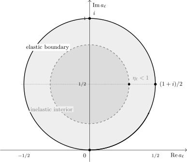
For $a_\ell=(S_\ell-1)/(2i)$, elastic scattering with $\eta_\ell=1$ lies on the outer circle, while an elastic element with $\eta_\ell\lt1$ lies inside it. The points $a_\ell=0$, $(1+i)/2$, and $i$ correspond to elastic phase shifts $\delta_\ell=0$, $\pi/4$, and $\pi/2$.

The figure is convention dependent only in its choice of normalized amplitude. The underlying statement that the full $S$-matrix is unitary is convention independent.

Bounds on Partial Cross Sections

For distinguishable spinless particles in the convention above, the elastic contribution of one partial wave is

$$\sigma_{\ell}^{\mathrm{el}} = \frac{4\pi}{k^2} (2\ell+1) \lvert a_\ell\rvert^2.$$

Because the unitarity disk implies

$$\lvert a_\ell\rvert\le1,$$

each channel obeys

$$\sigma_{\ell}^{\mathrm{el}} \le \frac{4\pi}{k^2} (2\ell+1).$$

The total and reaction contributions in the same partial wave are

$$\sigma_{\ell}^{\mathrm{tot}} = \frac{4\pi}{k^2} (2\ell+1) \operatorname{Im}a_\ell$$

and

$$\begin{aligned} \sigma_{\ell}^{\mathrm{reac}} &= \sigma_{\ell}^{\mathrm{tot}} - \sigma_{\ell}^{\mathrm{el}} \\ &= \frac{\pi}{k^2} (2\ell+1) \left( 1-\eta_\ell^2 \right). \end{aligned}$$

Therefore

$$\sigma_{\ell}^{\mathrm{reac}} \le \frac{\pi}{k^2} (2\ell+1).$$

Two limiting points are worth separating:

• elastic saturation: $\eta_\ell=1$ and $\delta_\ell=\pi/2$ give $a_\ell=i$ and saturate the elastic bound;
• complete absorption: $\eta_\ell=0$ gives $a_\ell=i/2$, with equal elastic-diffraction and reaction contributions.

For complete absorption,

$$\sigma_{\ell}^{\mathrm{el}} = \sigma_{\ell}^{\mathrm{reac}} = \frac{\pi}{k^2} (2\ell+1).$$

Absorption therefore does not eliminate elastic scattering. The sharp removal of part of an incoming wave produces diffractive elastic flux.

A channel bound is not a total bound

Summing the individual upper bound over infinitely many $\ell$ would diverge. Unitarity alone does not provide a finite bound on the total cross section without additional information about range, analyticity, energy, or which angular momenta couple appreciably.

For a short-range interaction of range $R$, the impact-parameter estimate

$$b \simeq \frac{\ell+1/2}{k}$$

suggests that the important channels satisfy roughly

$$\ell\lesssim kR.$$

Only after such dynamical input is supplied does the sum produce a geometric cross-section scale. Identical particles, spin, and coupled total-angular-momentum channels change degeneracy factors and which partial waves are allowed.

Partial-Wave Cross Sections owns the Legendre-orthogonality derivation, the complete elastic, reaction, and total sums, threshold scaling, and hard-sphere and black-disk examples. The present page owns the unitarity bounds that constrain those sums.

At low energy, the $s$ wave often dominates. Its elastic bound,

$$\sigma_0^{\mathrm{el}} \le \frac{4\pi}{k^2},$$

is reached near a short-range threshold pole when the scattering length is much larger than the interaction range. Low-Energy Scattering develops that regime.

More Than One Open Channel

At fixed energy and fixed conserved quantum numbers, a multichannel block obeys

$$S^{(J)\dagger}S^{(J)} = I.$$

For an incoming channel $\alpha$,

$$\left| S_{\alpha\alpha}^{(J)} \right|^2 + \sum_{\beta\ne\alpha} \left| S_{\beta\alpha}^{(J)} \right|^2 = 1.$$

It follows that

$$\left| S_{\alpha\alpha}^{(J)} \right| \le1.$$

Writing the elastic element as

$$S_{\alpha\alpha}^{(J)} = \eta_\alpha^{(J)} e^{2i\delta_\alpha^{(J)}}$$

does not mean the full block has become nonunitary. The deficit

$$1- \left( \eta_\alpha^{(J)} \right)^2$$

is exactly the probability carried by the other open channels in that column.

Projecting out channels

Let $P$ project onto channels retained in a model and let $Q=I-P$. The retained subblock is

$$S_P=PSP.$$

Using full-space unitarity,

$$\begin{aligned} S_P^\dagger S_P &= P - PS^\dagger QSP. \end{aligned}$$

For every retained state $\lvert\phi\rangle$,

$$\langle\phi\lvert PS^\dagger QSP \rvert\phi\rangle = \left\| QSP\lvert\phi\rangle \right\|^2 \ge0.$$

The projected matrix is therefore contractive rather than unitary whenever probability enters the omitted sector. This is the operator meaning of absorption in an optical potential or loss in a reduced reaction model.

An effective non-Hermitian Hamiltonian can represent that loss faithfully, but it should not be confused with a fundamental violation of probability conservation. Unitarity is recovered when the environment or eliminated channels are restored.

Perturbative Unitarity

A truncated amplitude need not be exactly unitary. It must satisfy unitarity through the order being claimed.

Introduce a coupling parameter:

$$\mathcal T = \lambda\mathcal T_1 + \lambda^2\mathcal T_2 + O(\lambda^3).$$

Substitute this expansion into

$$i \left( \mathcal T^\dagger-\mathcal T \right) = \mathcal T^\dagger\mathcal T.$$

At first order,

$$i \left( \mathcal T_1^\dagger-\mathcal T_1 \right) = 0.$$

At second order,

$$i \left( \mathcal T_2^\dagger-\mathcal T_2 \right) = \mathcal T_1^\dagger\mathcal T_1.$$

Thus the leading transition amplitude can be real in an appropriate elastic convention, while the next order must develop the imaginary part generated by the square of the leading amplitude. This is why a real first Born amplitude and a nonzero order-$\lambda^2$ cross section are consistent. Born Series derives the corresponding on-shell second-order term.

Failure of the order-$\lambda^2$ identity can reveal:

• a missing intermediate channel;
• an incorrect $i0$ prescription;
• inconsistent phase-space or state normalization;
• double counting between an iterated interaction and a matched kernel;
• a regulator or numerical discretization that does not preserve the relevant adjoint relation.

Enforcing Unitarity Is Not the Same as Deriving Dynamics

A Hermitian reaction matrix $K$ can be mapped to a unitary scattering matrix through

$$S = \left( I+iK \right) \left( I-iK \right)^{-1}.$$

Indeed, $K^\dagger=K$ implies $S^\dagger S=I$. The associated partial-wave amplitude is

$$a = K \left( I-iK \right)^{-1}.$$

For one elastic channel, choosing

$$K_\ell=\tan\delta_\ell$$

reproduces $S_\ell=e^{2i\delta_\ell}$.

This construction is useful for parameterization and controlled resummation. It does not prove that an approximate $K$ contains the correct left-hand singularities, thresholds, channel couplings, or pole residues. A formula can satisfy the unitarity circle exactly and still be physically inaccurate.

Numerical and Experimental Checks

For a computed channel matrix at energy $E$, define the unitarity residual

$$\Delta_U(E) = S^\dagger(E)S(E)-I.$$

Useful scalar diagnostics include

$$\lVert\Delta_U\rVert_2, \qquad \lVert\Delta_U\rVert_{\mathrm F},$$

and the maximum column deficit

$$\epsilon_{\mathrm{col}} = \max_\alpha \left| 1- \sum_\beta \lvert S_{\beta\alpha}\rvert^2 \right|.$$

The choice of norm and channel basis should be reported. A small matrix residual does not guarantee that the underlying dynamics is accurate; it only shows consistency with unitarity in the represented space.

Additional checks are:

• compare incoming and outgoing probability current at a large matching surface;
• verify that each elastic partial wave lies on the unitary circle;
• verify that an inelastic elastic element lies inside the disk by the amount carried by explicit reaction channels;
• check the optical theorem with the same normalization and channel sum;
• vary grid spacing, box size, matching radius, regulator, and channel cutoff;
• confirm perturbative identities at the order retained rather than demanding exact equality from a truncated series.

Experimental partial-wave analyses often impose unitarity while fitting data. This reduces the allowed parameter space, but model dependence remains in truncation, background parameterization, channel completeness, detector unfolding, and analytic continuation.

QFT Bridge

Relativistic field theory uses the same operator identity with a different state space and normalization. A common convention is

$$\begin{aligned} \langle f\lvert S-I\rvert i\rangle ={}& i(2\pi)^4 \delta^{(4)}(P_f-P_i) \\ &\times \mathcal M_{fi}. \end{aligned}$$

After the overall delta function is removed consistently, unitarity gives schematically

$$2\, \operatorname{Im} \mathcal M_{ii} = \sum_X \int d\Phi_X\, \left| \mathcal M_{Xi} \right|^2.$$

The sum includes every allowed on-shell multiparticle state, together with spin sums, symmetry factors, and Lorentz-invariant phase space. Diagrammatic cutting rules calculate these discontinuities order by order. They are an implementation of unitarity, not an additional conservation law.

QFT Bridge: Optical Theorem and Unitarity owns the relativistic translation and cutting interpretation.

Common Mistakes

• Requiring $\lvert S_{\alpha\alpha}\rvert=1$ when inelastic channels are open.
• Calling a reduced elastic subblock nonunitary without checking omitted channels.
• Summing channel amplitudes normalized to equal amplitude as though they carried equal flux.
• Squaring continuum delta functions instead of using packets or stripping conservation factors consistently.
• Mixing the conventions $S=I+i\mathcal T$ and $S=I-2\pi i\,\delta(E_f-E_i)T$.
• Treating a partial-wave bound as a finite bound on the total cross section without a range or angular-momentum cutoff.
• Demanding exact unitarity from a finite perturbative truncation instead of checking it order by order.
• Assuming that an exactly unitary parameterization is automatically a correct dynamical model.
• Interpreting loss from a non-Hermitian effective model as destruction of probability in the enlarged closed system.

Exercises

Derive the transition-operator identity

Starting from $S=I+i\mathcal T$, derive the unitarity relation and its diagonal matrix element.

Solution

Expand:

$$\begin{aligned} S^\dagger S &= \left( I-i\mathcal T^\dagger \right) \left( I+i\mathcal T \right) \\ &= I + i \left( \mathcal T-\mathcal T^\dagger \right) + \mathcal T^\dagger\mathcal T. \end{aligned}$$

Setting this equal to $I$ gives

$$i \left( \mathcal T^\dagger-\mathcal T \right) = \mathcal T^\dagger\mathcal T.$$

Taking the matrix element in $\lvert i\rangle$ and inserting

$$I=\sum_n\lvert n\rangle\langle n\rvert$$

on the right gives

$$2\, \operatorname{Im}\mathcal T_{ii} = \sum_n \lvert\mathcal T_{ni}\rvert^2.$$

Prove the unitarity-circle equation

Let

$$a = e^{i\delta}\sin\delta.$$

Show that $a$ lies on a circle of radius $1/2$ centered at $i/2$.

Solution

The real and imaginary parts are

$$x = \sin\delta\cos\delta, \qquad y = \sin^2\delta.$$

Then

$$\begin{aligned} x^2 + \left( y-\frac{1}{2} \right)^2 &= \sin^2\delta\cos^2\delta \\ &\quad+ \left( \sin^2\delta-\frac{1}{2} \right)^2 \\ &= \frac{1}{4}. \end{aligned}$$

Equivalently, elastic unitarity gives $y=\lvert a\rvert^2=x^2+y^2$, which rearranges to the same circle.

Separate elastic scattering from reaction loss

For

$$S_\ell = \eta_\ell e^{2i\delta_\ell},$$

show that

$$\sigma_\ell^{\mathrm{reac}} = \frac{\pi}{k^2} (2\ell+1) \left( 1-\eta_\ell^2 \right).$$

What happens at complete absorption?

Solution

With $a_\ell=(S_\ell-1)/(2i)$,

$$\operatorname{Im}a_\ell - \lvert a_\ell\rvert^2 = \frac{1-\eta_\ell^2}{4}.$$

Subtracting the elastic cross section from the total partial cross section gives

$$\begin{aligned} \sigma_\ell^{\mathrm{reac}} &= \frac{4\pi}{k^2} (2\ell+1) \left( \operatorname{Im}a_\ell - \lvert a_\ell\rvert^2 \right) \\ &= \frac{\pi}{k^2} (2\ell+1) \left( 1-\eta_\ell^2 \right). \end{aligned}$$

At complete absorption, $\eta_\ell=0$ and $a_\ell=i/2$. The elastic and reaction contributions are equal:

$$\sigma_\ell^{\mathrm{el}} = \sigma_\ell^{\mathrm{reac}} = \frac{\pi}{k^2} (2\ell+1).$$

Quantify loss from a projected channel space

Let $P+Q=I$, $PQ=0$, and $S^\dagger S=I$. Show that $S_P=PSP$ is contractive and identify its missing probability.

Solution

Insert $P=I-Q$ between $S^\dagger$ and $S$:

$$\begin{aligned} S_P^\dagger S_P &= PS^\dagger PSP \\ &= PS^\dagger \left( I-Q \right) SP \\ &= P - PS^\dagger QSP. \end{aligned}$$

For a retained incoming state $\lvert\phi\rangle=P\lvert\phi\rangle$,

$$\begin{aligned} \lVert\phi\rVert^2 - \lVert S_P\phi\rVert^2 &= \langle\phi\lvert PS^\dagger QSP \rvert\phi\rangle \\ &= \lVert QSP\phi\rVert^2 \ge0. \end{aligned}$$

The norm lost from the retained sector is exactly the probability scattered into the omitted $Q$ channels.

Check unitarity through second order

Suppose

$$\mathcal T = \lambda\mathcal T_1 + \lambda^2\mathcal T_2 + O(\lambda^3).$$

Derive the constraints at orders $\lambda$ and $\lambda^2$.

Solution

Substitution into

$$i \left( \mathcal T^\dagger-\mathcal T \right) = \mathcal T^\dagger\mathcal T$$

gives, at first order,

$$i \left( \mathcal T_1^\dagger-\mathcal T_1 \right) = 0.$$

Thus $\mathcal T_1$ is Hermitian on the open-channel shell. At second order,

$$i \left( \mathcal T_2^\dagger-\mathcal T_2 \right) = \mathcal T_1^\dagger\mathcal T_1.$$

The anti-Hermitian part of the second-order amplitude is fixed by products of first-order amplitudes into all on-shell intermediate channels.

Verify the K-matrix map

Let $K^\dagger=K$ and

$$S = \left( I+iK \right) \left( I-iK \right)^{-1}.$$

Show that $S$ is unitary.

Solution

Because both factors are functions of $K$, they commute. Hermiticity gives

$$S^\dagger = \left( I+iK \right)^{-1} \left( I-iK \right).$$

Therefore

$$\begin{aligned} S^\dagger S ={}& \left( I+iK \right)^{-1} \left( I-iK \right) \\ &\times \left( I+iK \right) \left( I-iK \right)^{-1} \\ ={}& I. \end{aligned}$$

The same calculation gives $SS^\dagger=I$.

References

• J. R. Taylor, Scattering Theory: The Quantum Theory of Nonrelativistic Collisions, Dover, 2006, Chapters 3 and 4.
• R. G. Newton, Scattering Theory of Waves and Particles, 2nd ed., Springer, 1982, Chapters 5, 10, and 11.
• M. L. Goldberger and K. M. Watson, Collision Theory, Wiley, 1964, Chapters 3 and 4.
• C. J. Joachain, Quantum Collision Theory, 3rd ed., North-Holland, 1983, Chapters 3 and 7.
• Particle Data Group, “Resonances,” Review of Particle Physics (2023), PDF.
• B. Zwiebach, “Chapter 7: Scattering,” MIT OpenCourseWare 8.06 Quantum Physics III (2018), course note.