T-Matrix

The transition operator $T$ is the interaction-dependent part of scattering. The S-Matrix maps complete incoming asymptotic data to outgoing data; the $T$-matrix removes the identity contribution and packages the amplitudes generated by the interaction.

The same letter is also used for transmission probability and, in some sources, time ordering. Here $T(z)$ always means the nonrelativistic scattering transition operator. Transmission probabilities carry an explicit label when ambiguity is possible, and time ordering is written $\mathcal T$.

Fix the Convention First

Let

$$H=H_0+V,$$

and use delta-normalized relative-momentum states

$$\begin{aligned} \langle\mathbf r\vert\mathbf k\rangle &= \frac{ e^{i\mathbf k\cdot\mathbf r} }{ (2\pi)^{3/2} }, \\ \langle\mathbf k'\vert\mathbf k\rangle &= \delta^{(3)} \left( \mathbf k'-\mathbf k \right). \end{aligned}$$

For free relative motion,

$$E_{\mathbf k} = \frac{\hbar^2k^2}{2\mu},$$

where $\mu$ is the reduced mass. In this normalization, the stationary relation between $S$ and the outgoing transition operator is

$$\begin{aligned} \langle\mathbf k'\lvert S \rvert\mathbf k\rangle ={}& \delta^{(3)} \left( \mathbf k'-\mathbf k \right) \\ &- 2\pi i\, \delta \left( E_{\mathbf k'}-E_{\mathbf k} \right) \\ &\quad\times \langle\mathbf k'\lvert T(E_{\mathbf k}+i0) \rvert\mathbf k\rangle. \end{aligned}$$

For energy-normalized channels, the same convention reads

$$\begin{aligned} \langle E',\beta\lvert S \rvert E,\alpha\rangle ={}& \delta(E'-E) \\ &\times \left[ \delta_{\beta\alpha} - 2\pi i\, T_{\beta\alpha}(E) \right]. \end{aligned}$$

The energy delta function belongs to the $S$-matrix element, not to the reduced fixed-energy matrix $T_{\beta\alpha}(E)$. With no interaction, $S=I$ and $T=0$.

Other normalizations move factors of $2\pi$, $\hbar$, masses, velocities, and delta functions. Every isolated formula for $T$ is incomplete until the state normalization and the definition of $S$ are stated.

Operator Definition

For complex energy $z$ away from the spectrum of $H_0$, define the free resolvent

$$G_0(z) = \frac{1}{z-H_0}.$$

The transition operator satisfies

$$T(z) = V + V G_0(z)T(z).$$

There is also a left form,

$$T(z) = V + T(z)G_0(z)V.$$

When the relevant inverses exist,

$$\begin{aligned} T(z) &= \left[ I-VG_0(z) \right]^{-1}V, \\ &= V \left[ I-G_0(z)V \right]^{-1}. \end{aligned}$$

The operator order matters because $V$ and $G_0$ need not commute. The full resolvent

$$G(z) = \frac{1}{z-H}$$

is related to $T$ by

$$G(z) = G_0(z) + G_0(z)T(z)G_0(z),$$

and equivalently

$$T(z) = V + V G(z)V.$$

Thus $T$ is not merely the potential. It contains every repeated interaction separated by free propagation.

Physical outgoing scattering uses the boundary value

$$T^{(+)}(E) = T(E+i0).$$

The infinitesimal prescription selects outgoing radiation. It is a boundary value across the continuous spectrum, not a small physical absorption constant.

Relation to Scattering States

The outgoing Lippmann–Schwinger state obeys

$$\lvert\psi_{\mathbf k}^{(+)}\rangle = \lvert\mathbf k\rangle + G_0^{(+)}(E_{\mathbf k}) V \lvert\psi_{\mathbf k}^{(+)}\rangle.$$

Multiplying by $V$ and comparing with the defining equation for $T$ gives

$$T^{(+)}(E_{\mathbf k}) \lvert\mathbf k\rangle = V \lvert\psi_{\mathbf k}^{(+)}\rangle.$$

Therefore the transition matrix element has two equivalent distorted-wave forms:

$$\begin{aligned} \langle\mathbf k'\lvert T^{(+)}(E_{\mathbf k}) \rvert\mathbf k\rangle &= \langle\mathbf k'\lvert V \rvert\psi_{\mathbf k}^{(+)}\rangle, \\ &= \langle\psi_{\mathbf k'}^{(-)} \lvert V \rvert\mathbf k\rangle \end{aligned}$$

when the external states are on the same energy shell and $V$ is self-adjoint. The first form builds the interaction into the initial state; the second builds it into the final test state.

Lippmann–Schwinger Equation owns the exact coordinate-space state equation, and Green Function for Scattering owns the outgoing-kernel and far-field derivation. This page owns the transition operator extracted from them.

From Matrix Elements to the Scattering Amplitude

For the normalized momentum kets fixed above, the elastic amplitude is

$$\begin{aligned} f( \mathbf k'\leftarrow\mathbf k ) = - \frac{4\pi^2\mu}{\hbar^2} \langle\mathbf k'\lvert T^{(+)}(E_{\mathbf k}) \rvert\mathbf k\rangle, \end{aligned}$$

with

$$\lvert\mathbf k'\rvert = \lvert\mathbf k\rvert = k.$$

The differential cross section in a single elastic channel is then

$$\frac{d\sigma}{d\Omega} = \left| f( \mathbf k'\leftarrow\mathbf k ) \right|^2.$$

The coefficient looks different if one starts from a coordinate-space wave with unit incident amplitude,

$$\psi_{\mathbf k}^{(+)}(\mathbf r) \sim e^{i\mathbf k\cdot\mathbf r} + f(\mathbf k'\leftarrow\mathbf k) \frac{e^{ikr}}{r}.$$

In that convention,

$$\begin{aligned} f( \mathbf k'\leftarrow\mathbf k ) ={}& - \frac{\mu}{2\pi\hbar^2} \\ &\times \int d^3r\, e^{-i\mathbf k'\cdot\mathbf r} V(\mathbf r) \psi_{\mathbf k}^{(+)}(\mathbf r). \end{aligned}$$

The two formulas agree because the normalized ket wavefunction carries a factor $(2\pi)^{-3/2}$ in both the incident state and the final-state bra. Comparing coefficients without carrying those factors is a common source of apparent contradictions.

For several channels, the relation between $T_{\beta\alpha}$ and $f_{\beta\alpha}$ depends on the channel normalization, reduced masses, and asymptotic velocities. Unit-flux normalization hides the velocity factors inside the states; other conventions display the factor $v_\beta/v_\alpha$ in the cross section.

Local Potentials and Momentum Transfer

For a local potential, define

$$\widetilde V(\mathbf q) = \int d^3r\, e^{-i\mathbf q\cdot\mathbf r} V(\mathbf r),$$

with momentum transfer

$$\mathbf q = \mathbf k'-\mathbf k.$$

The delta-normalized plane-wave matrix element is

$$\langle\mathbf k'\lvert V \rvert\mathbf k\rangle = \frac{ \widetilde V(\mathbf q) }{ (2\pi)^3 }.$$

Replacing $T$ by $V$ gives the first Born amplitude

$$f^{(1)}(\mathbf q) = - \frac{\mu}{2\pi\hbar^2} \widetilde V(\mathbf q).$$

The simple Fourier-transform rule is therefore the first term of the transition operator, not the definition of exact scattering. First Born Approximation owns its applications and validity criteria.

For a nonlocal interaction $V(\mathbf r,\mathbf r')$, the potential matrix element depends separately on incoming and outgoing momenta. Momentum-transfer dependence alone is no longer enough.

Born Expansion and Repeated Scattering

Formal iteration of the operator equation gives

$$\begin{aligned} T(z) ={}& V + V G_0(z)V \\ &+ V G_0(z)V G_0(z)V + \cdots. \end{aligned}$$

This identifies the exact $T$-matrix as a resummation of repeated interactions when the series is meaningful. Born Series is the canonical home for coupling-order bookkeeping, the second Born integral, convergence bounds, perturbative unitarity, and failure near poles. The exact operator equation and inverse identities on this page remain useful even where their Neumann expansion diverges.

Exact Resummation for a Separable Potential

A rank-one separable interaction makes the resummation explicit:

$$V = \lambda \lvert g\rangle \langle g\rvert.$$

Use the ansatz

$$T(z) = \lvert g\rangle \tau(z) \langle g\rvert.$$

Substitution into $T=V+VG_0T$ gives

$$\tau(z) = \lambda + \lambda I(z) \tau(z),$$

where

$$I(z) = \langle g\lvert G_0(z) \rvert g\rangle.$$

Thus

$$\tau(z) = \frac{\lambda}{ 1-\lambda I(z) }.$$

Expanding the denominator reproduces

$$\tau = \lambda + \lambda^2 I + \lambda^3 I^2 + \cdots.$$

The exact denominator shows what a finite Born truncation misses. A zero of $1-\lambda I(z)$ produces a pole associated, depending on its location and sheet, with a bound state, virtual state, or resonance.

On Shell, Half On Shell, and Off Shell

Write a momentum-space element as

$$T( \mathbf k',\mathbf k;z ) = \langle\mathbf k'\lvert T(z) \rvert\mathbf k\rangle.$$

For elastic scattering at physical energy $E$:

• on shell: $z=E+i0$ and $E_{\mathbf k'}=E_{\mathbf k}=E$;
• half on shell: one external free energy equals $E$, while the other does not;
• off shell: neither external free energy is constrained to equal $E$.

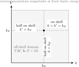
At fixed elastic energy $E$, the physical on-shell point in the $(k,k')$ magnitude plane is $k=k'=k_E$. The dashed lines are half-on-shell sets, and the surrounding domain is off shell. At the on-shell point, the directions $\hat{\mathbf k}$ and $\hat{\mathbf k}'$ still vary and carry the angular dependence.

Only on-shell elements enter the asymptotic $S$-matrix and isolated two-body cross sections. Half-on-shell and off-shell elements are nevertheless useful inside integral equations, few-body kernels, effective interactions, and numerical schemes.

Their usefulness does not make them separately observable. Scattering-equivalent unitary transformations can change off-shell matrix elements while leaving the on-shell $S$-matrix unchanged. In a many-body problem, induced many-body interactions and transformed current operators must be carried along consistently. Experimental data therefore do not determine a unique off-shell $T$-matrix without additional representation choices.

Unitarity Constraint

For self-adjoint $V$ and real $E$ above threshold,

$$T^{(-)}(E) = T^{(+)}(E)^\dagger.$$

The two boundary values obey

$$\begin{aligned} T^{(+)}(E) - T^{(-)}(E) ={}& - 2\pi i\, T^{(-)}(E) \\ &\times \delta(E-H_0) \\ &\times T^{(+)}(E). \end{aligned}$$

This follows from

$$G_0^{(+)}(E) - G_0^{(-)}(E) = - 2\pi i\, \delta(E-H_0).$$

Taking a diagonal momentum-space matrix element gives, schematically,

$$\begin{aligned} & 2\, \operatorname{Im} \langle\mathbf k\lvert T^{(+)} \rvert\mathbf k\rangle \\ &\quad= - 2\pi \int d^3k'\, \delta( E_{\mathbf k'}-E_{\mathbf k} ) \\ &\qquad\times \left| \langle\mathbf k'\lvert T^{(+)} \rvert\mathbf k\rangle \right|^2. \end{aligned}$$

The negative sign is correct for the convention $S=I-2\pi i\,\delta(E_f-E_i)T$. Since $f$ is proportional to $-T$, the corresponding forward amplitude has the sign required by the optical theorem. Changing the definition of $T$ changes this intermediate sign, not the observable relation.

When several channels are open, the resolution of identity includes a sum over every open channel and its phase-space measure. Omitting a channel makes the retained subblock appear nonunitary. Unitarity owns the channel-space consequences and bounds, while Optical Theorem develops the observable forward-scattering statement.

Analytic Structure

The operator $T(z)$ inherits branch cuts from the continuum resolvent and poles from the failure of

$$I-VG_0(z)$$

to be invertible. Below threshold on the physical sheet, a pole can represent a bound state. Analytic continuation through a continuum cut reaches sheets on which virtual-state and resonance poles may occur.

The pole residue factorizes for an isolated simple pole:

$$T(z) \sim \frac{ \lvert\Gamma_R\rangle \langle\widetilde\Gamma_R\rvert }{ z-z_R }.$$

The precise relation between the residue, a normalizable bound state, or a Gamow resonance depends on the pole location and analytic sheet. Bound States and Scattering Poles owns that classification.

Numerical Use

In momentum space, one solves

$$\begin{aligned} T( \mathbf k',\mathbf k;E ) ={}& V( \mathbf k',\mathbf k ) \\ &+ \int d^3p\, V( \mathbf k',\mathbf p ) \\ &\quad\times \frac{ T( \mathbf p,\mathbf k;E ) }{ E-E_{\mathbf p}+i0 }. \end{aligned}$$

For central interactions, partial-wave projection reduces the three-dimensional equation to coupled one-dimensional integral equations. Practical methods separate the principal value from the on-shell delta term, subtract the singularity analytically, or solve at complex energy and take a controlled boundary limit.

Contact interactions and singular short-distance potentials can make the momentum integral ultraviolet divergent. A regulator alone is not a prediction; its parameters must be matched so observables are regulator independent within the claimed accuracy.

Useful numerical checks include:

• recovering $T=V$ at first Born order;
• reproducing the no-interaction limit;
• checking reciprocity when time-reversal symmetry applies;
• testing the optical theorem or fixed-energy unitarity;
• varying momentum cutoff and grid resolution;
• locating poles consistently from more than one observable or continuation method.

QFT Convention Warning

Quantum field theory often writes

$$\begin{aligned} \langle f\lvert S\rvert i\rangle ={}& \langle f\vert i\rangle \\ &+ i(2\pi)^4 \delta^{(4)}(P_f-P_i) \mathcal M_{fi}. \end{aligned}$$

The invariant amplitude $\mathcal M$ is not the nonrelativistic potential-scattering matrix element $\langle\mathbf k'|T|\mathbf k\rangle$. Relativistic one-particle normalization, multiparticle phase space, particle production, spin sums, and flux conventions all differ.

Likewise, the time-ordering symbol $\mathcal T$ in a Dyson series is an ordering operation, not this transition operator. The conceptual analogy between a Born term and a tree-level exchange is useful only after matching the full amplitude and kinematics. QFT Bridge: Born Approximation and Tree Level states that boundary carefully.

Practical Workflow

1. Specify $H_0$, $V$, and the asymptotic channel basis.
2. Record momentum, energy, or unit-flux normalization.
3. Choose $T^{(+)}$, $T^{(-)}$, or complex-energy $T(z)$ and state the boundary condition.
4. Solve the operator or projected integral equation.
5. Put external states on shell only when forming the physical $S$-matrix or cross section.
6. Convert the on-shell element to $f$ with the matching normalization coefficient.
7. Sum all open channels when checking unitarity.
8. Test cutoff, grid, and truncation dependence before interpreting off-shell structure or poles.

Common Mistakes

• Treating $T$ as a transmission probability.
• Identifying $T$ with $V$ beyond first Born order.
• Omitting the identity part or energy delta function when reconstructing $S$.
• Mixing unit-amplitude waves with delta-normalized kets in the amplitude coefficient.
• Calling an intermediate momentum on shell merely because the external energy is physical.
• Treating an off-shell matrix element as a uniquely measurable quantity.
• Dropping the $i0$ prescription in a continuum integral.
• Truncating the Born series near a pole without checking convergence.
• Comparing the sign of $\operatorname{Im}T$ across different $S$-matrix conventions.
• Equating the nonrelativistic $T$-matrix with the QFT invariant amplitude $\mathcal M$.

Cross-Links

• Scattering Theory
• S-Matrix
• Scattering Amplitude
• Lippmann–Schwinger Equation
• Green Function for Scattering
• Born Series
• First Born Approximation
• Optical Theorem
• Bound States and Scattering Poles
• Energy Green Function
• Scattering Convention Dictionary
• QFT Bridge: Born Approximation and Tree Level

References

1. B. A. Lippmann and J. Schwinger, “Variational principles for scattering processes. I,” Physical Review 79, 469–480 (1950).
2. M. Gell-Mann and M. L. Goldberger, “The formal theory of scattering,” Physical Review 91, 398–408 (1953).
3. H. Ekstein, “Equivalent Hamiltonians in scattering theory,” Physical Review 117, 1590–1595 (1960).
4. J. R. Taylor, Scattering Theory: The Quantum Theory of Nonrelativistic Collisions, Dover (2006).
5. R. G. Newton, Scattering Theory of Waves and Particles, 2nd ed., Dover (2002).
6. M. L. Goldberger and K. M. Watson, Collision Theory, Dover (2004).
7. C. J. Joachain, Quantum Collision Theory, 3rd ed., North-Holland (1983).
8. M. Reed and B. Simon, Methods of Modern Mathematical Physics, Vol. III: Scattering Theory, Academic Press (1979).

Exercises

1. Connect the transition operator to the scattering state

Starting from

$$\lvert\psi_{\mathbf k}^{(+)}\rangle = \lvert\mathbf k\rangle + G_0^{(+)}V \lvert\psi_{\mathbf k}^{(+)}\rangle,$$

show that

$$T^{(+)} \lvert\mathbf k\rangle = V \lvert\psi_{\mathbf k}^{(+)}\rangle.$$

Solution

Multiply the scattering-state equation by $V$:

$$\begin{aligned} V \lvert\psi_{\mathbf k}^{(+)}\rangle ={}& V\lvert\mathbf k\rangle \\ &+ VG_0^{(+)} V \lvert\psi_{\mathbf k}^{(+)}\rangle. \end{aligned}$$

The vector $T^{(+)}\lvert\mathbf k\rangle$ obeys

$$T^{(+)}\lvert\mathbf k\rangle = V\lvert\mathbf k\rangle + VG_0^{(+)} T^{(+)}\lvert\mathbf k\rangle.$$

The two vectors solve the same integral equation with the same outgoing boundary value, so

$$T^{(+)} \lvert\mathbf k\rangle = V \lvert\psi_{\mathbf k}^{(+)}\rangle.$$

2. Recover the first Born normalization

Using

$$\langle\mathbf r\vert\mathbf k\rangle = (2\pi)^{-3/2} e^{i\mathbf k\cdot\mathbf r},$$

show that a local potential gives

$$\langle\mathbf k'\lvert V\rvert\mathbf k\rangle = (2\pi)^{-3} \widetilde V(\mathbf k'-\mathbf k),$$

and recover the stated first Born amplitude.

Solution

Insert position resolutions:

$$\begin{aligned} \langle\mathbf k'\lvert V\rvert\mathbf k\rangle ={}& \int d^3r\, \langle\mathbf k'\vert\mathbf r\rangle V(\mathbf r) \langle\mathbf r\vert\mathbf k\rangle, \\ ={}& \frac{1}{(2\pi)^3} \int d^3r\, e^{-i(\mathbf k'-\mathbf k)\cdot\mathbf r} V(\mathbf r), \\ ={}& \frac{ \widetilde V(\mathbf q) }{ (2\pi)^3 }. \end{aligned}$$

At first Born order, $T^{(1)}=V$. Therefore

$$\begin{aligned} f^{(1)}(\mathbf q) &= - \frac{4\pi^2\mu}{\hbar^2} \frac{ \widetilde V(\mathbf q) }{ (2\pi)^3 }, \\ &= - \frac{\mu}{2\pi\hbar^2} \widetilde V(\mathbf q). \end{aligned}$$

3. Sum the separable interaction

For

$$V=\lambda\lvert g\rangle\langle g\rvert,$$

substitute $T=\lvert g\rangle\tau\langle g\rvert$ into the transition-operator equation and solve for $\tau(z)$.

Solution

Substitution gives

$$\begin{aligned} \lvert g\rangle \tau \langle g\rvert ={}& \lambda \lvert g\rangle \langle g\rvert \\ &+ \lambda \lvert g\rangle \langle g\lvert G_0\rvert g\rangle \tau \langle g\rvert. \end{aligned}$$

Matching the scalar coefficients yields

$$\tau = \lambda + \lambda I\tau, \qquad I(z) = \langle g\lvert G_0(z)\rvert g\rangle.$$

Hence

$$\tau(z) = \frac{\lambda}{ 1-\lambda I(z) }.$$

4. Derive the transition-operator discontinuity

Use the two operator equations for $T^{(+)}$ and $T^{(-)}$ to show

$$\begin{aligned} T^{(+)}-T^{(-)} ={}& T^{(-)} \\ &\times \left( G_0^{(+)}-G_0^{(-)} \right) \\ &\times T^{(+)}. \end{aligned}$$

Then insert the resolvent discontinuity.

Solution

A standard two-potential identity follows by subtracting the two transition equations while preserving operator order:

$$\begin{aligned} T^{(+)}-T^{(-)} ={}& T^{(-)} \\ &\times \left( G_0^{(+)}-G_0^{(-)} \right) \\ &\times T^{(+)}. \end{aligned}$$

Using

$$G_0^{(+)}-G_0^{(-)} = -2\pi i\,\delta(E-H_0)$$

gives

$$\begin{aligned} T^{(+)}-T^{(-)} ={}& - 2\pi i\,T^{(-)} \\ &\times \delta(E-H_0) T^{(+)}. \end{aligned}$$

For self-adjoint dynamics, $T^{(-)}=T^{(+)\dagger}$, so this is the $T$-matrix form of unitarity.

5. Decide what is observable

At fixed elastic energy $E=\hbar^2k_E^2/(2\mu)$, classify the following matrix elements:

1. $T(\mathbf k',\mathbf k;E+i0)$ with $k'=k=k_E$;
2. the same element with $k=k_E$ but $k'\ne k_E$;
3. the same element with both magnitudes different from $k_E$.

Which enters an isolated two-body cross section directly?

Solution

The first element is on shell, although the directions of $\mathbf k$ and $\mathbf k'$ may differ. The second is half on shell because only the incoming free energy equals $E$. The third is off shell.

Only the first enters the asymptotic two-body $S$-matrix and cross section directly. Half-on-shell and off-shell elements can enter intermediate integral equations, but they depend on representation choices and are not separately fixed by scattering data.