S-Matrix

The scattering matrix compresses the entire collision into a map from freely propagating data in the remote past to freely propagating data in the remote future. It does not describe the detailed motion while the particles overlap. Instead, it answers the operational question: given a prepared incoming wave packet, what coherent superposition of outgoing channels will be observed after the interaction has ended?

This page is the canonical home for the nonrelativistic scattering operator. Scattering States and Boundary Conditions owns the construction of individual in and out states, while QFT Bridge: S-Matrix owns the translation to Fock space, relativistic normalization, and LSZ reduction.

Definition from Asymptotic States

Let

$$H=H_0+V,$$

where $H_0$ generates the chosen free channel dynamics and $V$ contains the interaction. The time-dependent Møller wave operators are

$$\Omega^{(\pm)} = \operatorname*{s-lim}_{t\to\mp\infty} e^{iHt/\hbar} e^{-iH_0t/\hbar}.$$

The sign labels a boundary condition, not the sign of the energy:

• $\Omega^{(+)}$ maps incoming free data in the distant past into the corresponding interacting scattering state;
• $\Omega^{(-)}$ maps outgoing free data in the distant future into that same physical scattering subspace.

For a physical scattering wave packet $\lvert\Psi\rangle$, write

$$\begin{aligned} \lvert\Psi\rangle &= \Omega^{(+)} \lvert\phi_{\mathrm{in}}\rangle, \\ \lvert\Psi\rangle &= \Omega^{(-)} \lvert\phi_{\mathrm{out}}\rangle. \end{aligned}$$

If the wave operators are isometric on the free scattering space, then

$$\lvert\phi_{\mathrm{out}}\rangle = \Omega^{(-)\dagger} \Omega^{(+)} \lvert\phi_{\mathrm{in}}\rangle.$$

The scattering operator is therefore

$$S = \Omega^{(-)\dagger} \Omega^{(+)}.$$

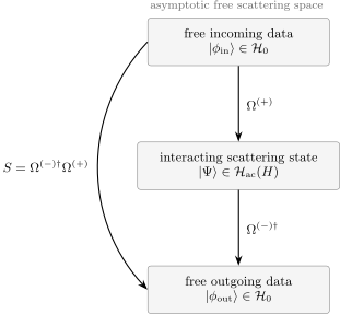
The two routes agree: $\lvert\phi_{\mathrm{out}}\rangle=S\lvert\phi_{\mathrm{in}}\rangle$ with $S=\Omega^{(-)\dagger}\Omega^{(+)}$. The operator $S$ acts on asymptotic free data; the wave operators connect those data to the absolutely continuous scattering subspace of $H$.

The corresponding channel matrix element is

$$\begin{aligned} S_{\beta\alpha} &= \langle\phi_\beta\lvert S \rvert\phi_\alpha\rangle, \\ &= \langle\psi_\beta^{(-)} \vert \psi_\alpha^{(+)}\rangle, \end{aligned}$$

where

$$\lvert\psi_\alpha^{(\pm)}\rangle = \Omega^{(\pm)} \lvert\phi_\alpha\rangle.$$

The plus state represents the prepared incoming channel, whereas the minus state tests a selected outgoing channel. Their overlap is an amplitude, so alternatives must be added coherently before probabilities are formed.

What Space the Operator Acts On

The notation $S$ can conceal three related objects:

1. the scattering operator on normalizable asymptotic wave packets;
2. its distribution-valued matrix elements between generalized energy or momentum eigenstates;
3. the finite-dimensional or countably infinite channel matrix $S(E)$ on a fixed energy shell.

The first is the mathematically clean starting point. Plane waves are useful generalized basis vectors, but they are not normalizable states. Delta functions in stationary matrix elements arise because the packet operator commutes with free time evolution; they should not be squared as ordinary numbers.

Bound states of $H$ are not asymptotic free channels. The wave operators map the free scattering space into the absolutely continuous subspace of the full Hamiltonian. If $P_{\mathrm{ac}}(H)$ projects onto that subspace, asymptotic completeness means

$$\operatorname{Ran}\Omega^{(+)} = \operatorname{Ran}\Omega^{(-)} = \operatorname{Ran}P_{\mathrm{ac}}(H).$$

This is stronger than merely assuming that the formal limits defining $\Omega^{(\pm)}$ exist. It says that every scattering state is accounted for by asymptotic channel data. Continuous Spectra and Rigged Hilbert Spaces: First Look provide the spectral background.

Energy-Shell Structure

The wave operators satisfy the intertwining relations

$$H\Omega^{(\pm)} = \Omega^{(\pm)}H_0.$$

Consequently,

$$H_0S=SH_0.$$

For a time-independent interaction, the scattering operator therefore preserves free energy. In an energy-normalized channel basis,

$$\langle E',\beta\lvert S \rvert E,\alpha\rangle = \delta(E'-E)\, S_{\beta\alpha}(E).$$

The delta function expresses energy conservation. The object $S(E)$ acts only among channels open at that energy. If the incoming packet has amplitudes $a_\alpha(E)$, the outgoing amplitudes are

$$b_\beta(E) = \sum_\alpha S_{\beta\alpha}(E) a_\alpha(E).$$

Thus $S(E)$ is not a time-evolution operator over a finite interval. It is an energy-resolved comparison between two asymptotic descriptions after the interacting evolution has been taken to infinite past and future.

Additional conserved quantities further block-diagonalize $S$. For a rotationally invariant two-body interaction, one can use total angular momentum and parity. For a translationally invariant isolated collision, total center-of-mass momentum is conserved. A fixed external target, by contrast, can absorb momentum, so its one-particle scattering operator need not commute with the projectile momentum.

Unitarity and Probability Conservation

For self-adjoint $H$ and $H_0$, existing wave operators are isometries on their initial scattering space:

$$\Omega^{(\pm)\dagger} \Omega^{(\pm)} = I.$$

If they are also asymptotically complete, then

$$\Omega^{(\pm)} \Omega^{(\pm)\dagger} = P_{\mathrm{ac}}(H).$$

These identities give

$$\begin{aligned} S^\dagger S &= \Omega^{(+)\dagger} P_{\mathrm{ac}}(H) \Omega^{(+)}, \\ &=I, \end{aligned}$$

and similarly $SS^\dagger=I$. Hence

$$S^\dagger S = SS^\dagger = I.$$

On a fixed energy shell, unitarity becomes

$$\sum_\beta S_{\beta\alpha}^*(E) S_{\beta\gamma}(E) = \delta_{\alpha\gamma}.$$

For a normalized packet incident in channel $\alpha$,

$$\sum_\beta \lvert S_{\beta\alpha}(E)\rvert^2 = 1.$$

This equation is probability conservation written in an orthonormal, unit-flux channel basis. It is the operator-level version of the surface-flux balance developed in Probability Current and Flux.

Unitarity takes this operator identity as its starting point and owns the transition-amplitude relation, partial-wave disk, inelasticity deficit, cross-section bounds, and perturbative tests.

The full open-channel matrix may be unitary even when an elastic element has magnitude below one. Probability then leaves that elastic channel but appears in other open channels. Apparent nonunitarity usually signals one of four things:

• some open channels were omitted;
• channel states were not flux normalized;
• an effective non-Hermitian optical potential deliberately absorbs probability;
• the wave operators are incomplete or inappropriate for the chosen long-range dynamics.

Identity Part and Transition Part

With no interaction and identical asymptotic conventions, $S=I$. It is useful to separate this no-collision contribution from the connected transition amplitude.

For energy-normalized channel states, one common nonrelativistic convention is

$$\begin{aligned} \langle E',\beta\lvert S \rvert E,\alpha\rangle ={}& \delta(E'-E) \\ &\times \left[ \delta_{\beta\alpha} - 2\pi i\, T_{\beta\alpha}(E) \right]. \end{aligned}$$

Equivalently, the energy-shell matrix is

$$S(E) = I_E - 2\pi i\,T(E)$$

in this convention. T-Matrix owns this transition operator, its exact normalization, and its on-shell versus off-shell matrix elements. It can be obtained from

$$T(E) = V + V G_0^{(+)}(E)T(E),$$

where

$$G_0^{(+)}(E) = \frac{1}{E-H_0+i0}.$$

This is the operator form behind the Lippmann–Schwinger Equation. The $S$-matrix is on shell: it connects asymptotic states with the same conserved energy. The operator $T(E)$ can also be evaluated between off-shell momenta inside integral equations, but those off-shell matrix elements are intermediate, convention-dependent objects rather than direct scattering observables.

Many QFT texts instead write

$$S=I+i\mathcal T.$$

The symbols $T$ and $\mathcal T$ then do not denote the same normalized object. Factors of $2\pi$, energy-momentum delta functions, state normalizations, signs, and powers of $\hbar$ may all move between definitions. Scattering Convention Dictionary should be consulted before comparing formulas.

In the schematic convention $S=I+i\mathcal T$, unitarity implies

$$i\left( \mathcal T^\dagger-\mathcal T \right) = \mathcal T^\dagger\mathcal T.$$

Taking a diagonal matrix element and inserting a complete set of open final states produces the optical theorem. The full derivation and its normalization-dependent factors belong in Optical Theorem.

Partial-Wave Eigenvalues

For a short-range central potential without spin, rotational invariance makes the energy-shell scattering matrix diagonal in $\ell$ and $m$:

$$\begin{aligned} \langle E',\ell',m'\lvert S \rvert E,\ell,m\rangle ={}& \delta(E'-E) \delta_{\ell'\ell} \delta_{m'm} \\ &\times S_\ell(E). \end{aligned}$$

The asymptotic reduced radial wave can be normalized as

$$\begin{aligned} u_\ell(k,r) \sim \frac{1}{2i} \Big[ & S_\ell(k) e^{i(kr-\ell\pi/2)} \\ &- e^{-i(kr-\ell\pi/2)} \Big]. \end{aligned}$$

The second exponential is incoming and the first is outgoing. In one-channel elastic scattering, unitarity gives $\lvert S_\ell\rvert=1$, so

$$S_\ell(k) = e^{2i\delta_\ell(k)}.$$

The factor of two follows directly from

$$\begin{aligned} \sin(x+\delta_\ell) = \frac{e^{-i\delta_\ell}}{2i} \Big[ & e^{2i\delta_\ell}e^{ix} \\ &- e^{-ix} \Big]. \end{aligned}$$

After an irrelevant overall phase is removed, fixing the incoming coefficient leaves the outgoing coefficient multiplied by $e^{2i\delta_\ell}$. Phase Shifts owns their physical interpretation and extraction.

For the amplitude convention

$$\psi(\mathbf r) \sim e^{ikz} + f(\theta) \frac{e^{ikr}}{r},$$

the partial-wave amplitude is

$$f(\theta) = \frac{1}{2ik} \sum_{\ell=0}^{\infty} (2\ell+1) \left( S_\ell-1 \right) P_\ell(\cos\theta).$$

The subtraction of $1$ removes the outgoing spherical component already contained in the incident plane wave. Partial-Wave Expansion derives the formula, while Differential and Total Cross Sections converts it into observables.

More Than One Open Channel

A channel includes all asymptotic labels needed to specify a free arrangement: particle species or internal states, relative momentum, orbital and spin quantum numbers, and any conserved total quantum numbers. At fixed energy, only channels with real asymptotic momentum carry flux to infinity.

Using unit-flux channel states, the open-channel matrix obeys

$$S^\dagger(E)S(E)=I_{\mathrm{open}}.$$

For a chosen partial wave, an elastic diagonal element is often parameterized as

$$\begin{aligned} S_{\alpha\alpha}^{(\ell)}(E) &= \eta_{\alpha\ell}(E) e^{2i\delta_{\alpha\ell}(E)}, \\ 0 &\le \eta_{\alpha\ell} \le1. \end{aligned}$$

The inelasticity $\eta_{\alpha\ell}$ is not evidence that the full theory violates unitarity. Rather,

$$\sum_{\beta\ne\alpha} \left| S_{\beta\alpha}^{(\ell)} \right|^2 = 1-\eta_{\alpha\ell}^2$$

when the column includes every open channel.

If coordinate-wave amplitudes rather than unit-flux amplitudes are used, channel velocities appear as weights. Rescaling each channel by the square root of its asymptotic velocity converts the weighted conservation law into ordinary matrix unitarity. Closed channels are absent from the asymptotic sum because they carry no flux, yet virtual excursions into them can strongly modify $S(E)$ and generate Feshbach resonances. Multichannel Scattering Preview develops that structure.

Symmetries, Rephasing, and Reciprocity

A symmetry shared by $H$ and $H_0$ constrains the scattering matrix. Rotational invariance produces angular-momentum blocks, parity separates even and odd sectors, and exchange symmetry restricts identical particles to bosonic or fermionic subspaces.

Channel phases remain conventional. Under

$$\lvert E,\alpha\rangle \longrightarrow e^{i\chi_\alpha(E)} \lvert E,\alpha\rangle,$$

the matrix transforms as

$$S_{\beta\alpha}(E) \longrightarrow e^{-i\chi_\beta(E)} S_{\beta\alpha}(E) e^{i\chi_\alpha(E)}.$$

Probabilities and consistently constructed interference observables are unchanged. A bare matrix entry should therefore never be quoted without specifying the channel basis and phase convention.

Time-reversal invariance can imply reciprocity relations between a process and its reversed process. The precise relation involves the antiunitary time-reversal operator and possible spin phase conventions; it is not simply the statement that every $S$-matrix is symmetric in every basis. Time Reversal gives the underlying antiunitary structure.

Wave Packets and Measured Probabilities

For a normalized incoming packet,

$$\lvert\phi_{\mathrm{in}}\rangle = \sum_\alpha \int dE\, a_\alpha(E) \lvert E,\alpha\rangle,$$

the outgoing packet is

$$\lvert\phi_{\mathrm{out}}\rangle = \sum_\beta \int dE\, b_\beta(E) \lvert E,\beta\rangle,$$

with $b_\beta(E)=\sum_\alpha S_{\beta\alpha}(E)a_\alpha(E)$. Unitarity ensures equality of the packet norms.

Experiments rarely reconstruct the full complex matrix directly. They measure probabilities or rates in finite angular, energy, spin, and channel bins. Cross sections divide those rates by incident flux; polarization and interference measurements can recover relative phases. This is why $S$ is richer than any single cross section but remains tied to operationally defined asymptotic preparations and detections.

Scope and Caveats

The standard construction above assumes time-independent, self-adjoint dynamics with suitable short-range asymptotics.

• Long-range forces. For an unscreened Coulomb potential, free Møller operators require modification because the asymptotic state accumulates a logarithmic Coulomb phase. Use Coulomb-distorted asymptotic dynamics rather than treating the failure as nonunitarity.
• Thresholds. The dimension and analytic behavior of $S(E)$ change when channels open or close. Square-root branch points and threshold laws require care.
• Bound states. Normalizable bound states do not appear as open asymptotic channels, although they influence analytic continuation and Levinson-type relations.
• Resonances. On the physical real axis a complete theory remains unitary; resonance poles appear only after analytic continuation to an unphysical sheet.
• Optical potentials. A negative imaginary potential intentionally removes flux from the retained subspace. Its reduced $S$-matrix is subunitary because eliminated reaction channels are not represented explicitly.
• Time-dependent driving. If the Hamiltonian is periodic rather than time independent, quasienergy replaces ordinary energy and Floquet sidebands become channels.

Coulomb Scattering treats the long-range exception, and Bound States and Scattering Poles owns the analytic continuation.

QFT Bridge

The structural statement

$$S_{fi} = \langle f,\mathrm{out} \vert i,\mathrm{in}\rangle$$

survives in relativistic quantum field theory. What changes is substantial: the asymptotic states live in Fock space, particle number can change, normalization is relativistic, Lorentz-invariant phase space replaces fixed-energy solid-angle counting, and LSZ reduction extracts amplitudes from field correlation functions.

Those changes are not normalization footnotes. They define a different realization of the same asymptotic idea. The canonical translation is QFT Bridge: S-Matrix.

Practical Checks

Before trusting an $S$-matrix calculation:

1. State $H_0$, $H$, and the asymptotic channel basis.
2. Specify plane-wave, momentum, energy, or unit-flux normalization.
3. Identify all open channels at the energy of interest.
4. Use boundary conditions appropriate to short- or long-range interactions.
5. Separate the identity contribution from the transition part consistently.
6. Check $S^\dagger S=I$ on the full open-channel space for self-adjoint dynamics.
7. Verify symmetry blocks, threshold behavior, and the no-interaction limit.
8. Translate amplitudes into cross sections only after flux and phase-space factors are fixed.

Common Mistakes

• Calling $S$ the finite-time evolution operator.
• Reversing $\Omega^{(+)}$ and $\Omega^{(-)}$ without also changing the convention for in and out states.
• Treating plane-wave matrix elements as ordinary finite-dimensional entries and squaring delta functions.
• Applying $S^\dagger S=I$ to an elastic subblock after inelastic channels have been omitted.
• Forgetting that velocity weights are hidden inside unit-flux channel normalization.
• Comparing $S=I-2\pi i\,T$ with $S=I+i\mathcal T$ as if $T=\mathcal T$.
• Writing $S_\ell=e^{i\delta_\ell}$ instead of $e^{2i\delta_\ell}$.
• Using free asymptotic states for an unscreened Coulomb interaction.
• Treating off-shell $T$-matrix elements as direct observables.
• Assuming time-reversal invariance makes $S$ symmetric in an arbitrary channel basis.

Cross-Links

• Scattering Theory
• Scattering States and Boundary Conditions
• Probability Current and Flux
• T-Matrix
• Lippmann–Schwinger Equation
• Partial-Wave Expansion
• Phase Shifts
• Optical Theorem
• Multichannel Scattering Preview
• One-Dimensional Scattering Revisited
• Scattering Convention Dictionary
• QFT Bridge: S-Matrix

References

1. C. Møller, General Properties of the Characteristic Matrix in the Theory of Elementary Particles, I, Matematisk-fysiske Meddelelser 23(1), 1–48 (1945).
2. M. Gell-Mann and M. L. Goldberger, “The formal theory of scattering,” Physical Review 91, 398–408 (1953).
3. B. A. Lippmann and J. Schwinger, “Variational principles for scattering processes. I,” Physical Review 79, 469–480 (1950).
4. J. R. Taylor, Scattering Theory: The Quantum Theory of Nonrelativistic Collisions, Dover (2006).
5. R. G. Newton, Scattering Theory of Waves and Particles, 2nd ed., Dover (2002).
6. M. Reed and B. Simon, Methods of Modern Mathematical Physics, Vol. III: Scattering Theory, Academic Press (1979).
7. M. L. Goldberger and K. M. Watson, Collision Theory, Dover (2004).
8. C. J. Joachain, Quantum Collision Theory, 3rd ed., North-Holland (1983).

Exercises

1. Recover the asymptotic map

Suppose

$$\lvert\Psi\rangle = \Omega^{(+)} \lvert\phi_{\mathrm{in}}\rangle = \Omega^{(-)} \lvert\phi_{\mathrm{out}}\rangle$$

and $\Omega^{(-)\dagger}\Omega^{(-)}=I$. Derive the map from the incoming to the outgoing free state.

Solution

Act with $\Omega^{(-)\dagger}$:

$$\begin{aligned} \Omega^{(-)\dagger} \lvert\Psi\rangle &= \Omega^{(-)\dagger} \Omega^{(+)} \lvert\phi_{\mathrm{in}}\rangle, \\ &= S \lvert\phi_{\mathrm{in}}\rangle. \end{aligned}$$

Using the second representation of $\lvert\Psi\rangle$ gives

$$\Omega^{(-)\dagger} \lvert\Psi\rangle = \lvert\phi_{\mathrm{out}}\rangle.$$

Therefore

$$\lvert\phi_{\mathrm{out}}\rangle = S \lvert\phi_{\mathrm{in}}\rangle.$$

2. Show that scattering conserves free energy

Use

$$H\Omega^{(\pm)} = \Omega^{(\pm)}H_0$$

to prove $H_0S=SH_0$. Explain the implication for stationary matrix elements.

Solution

Taking the adjoint of the minus intertwining relation gives

$$H_0\Omega^{(-)\dagger} = \Omega^{(-)\dagger}H.$$

Hence

$$\begin{aligned} H_0S &= H_0\Omega^{(-)\dagger}\Omega^{(+)}, \\ &= \Omega^{(-)\dagger}H\Omega^{(+)}, \\ &= \Omega^{(-)\dagger}\Omega^{(+)}H_0, \\ &= SH_0. \end{aligned}$$

Between generalized energy eigenstates,

$$(E'-E) \langle E',\beta\lvert S \rvert E,\alpha\rangle = 0.$$

Distributionally, the matrix element is therefore supported at $E'=E$ and contains $\delta(E'-E)$.

3. Prove unitarity from completeness

Assume

$$\Omega^{(\pm)\dagger}\Omega^{(\pm)}=I$$

and

$$\Omega^{(\pm)}\Omega^{(\pm)\dagger} = P_{\mathrm{ac}}(H).$$

Show both $S^\dagger S=I$ and $SS^\dagger=I$.

Solution

First,

$$\begin{aligned} S^\dagger S &= \Omega^{(+)\dagger} \Omega^{(-)} \Omega^{(-)\dagger} \Omega^{(+)}, \\ &= \Omega^{(+)\dagger} P_{\mathrm{ac}}(H) \Omega^{(+)}, \\ &= \Omega^{(+)\dagger}\Omega^{(+)}, \\ &=I. \end{aligned}$$

The projector can be removed on the third line because the range of $\Omega^{(+)}$ lies in the absolutely continuous subspace. Interchanging plus and minus gives

$$SS^\dagger=I.$$

Equal ranges of the two complete wave operators are the essential extra input.

4. Explain the doubled phase

Starting from $u_\ell(r)\propto\sin(x+\delta_\ell)$ with $x=kr-\ell\pi/2$, fix the coefficient of the incoming exponential and find the relative outgoing coefficient.

Solution

Write

$$\begin{aligned} \sin(x+\delta_\ell) &= \frac{ e^{i(x+\delta_\ell)} - e^{-i(x+\delta_\ell)} }{2i}, \\ &= \frac{e^{-i\delta_\ell}}{2i} \left[ e^{2i\delta_\ell}e^{ix} - e^{-ix} \right]. \end{aligned}$$

The prefactor is an irrelevant overall normalization and phase. Once the incoming coefficient of $e^{-ix}$ is fixed, the outgoing coefficient is

$$S_\ell=e^{2i\delta_\ell}.$$

5. Account for an inelastic channel

For an incoming partial-wave channel $\alpha$, suppose

$$S_{\alpha\alpha}^{(\ell)} = \eta_\ell e^{2i\delta_\ell}.$$

If exactly one other channel $\beta$ is open, determine $\lvert S_{\beta\alpha}^{(\ell)}\rvert^2$.

Solution

Column unitarity gives

$$\left| S_{\alpha\alpha}^{(\ell)} \right|^2 + \left| S_{\beta\alpha}^{(\ell)} \right|^2 = 1.$$

Since the elastic modulus is $\eta_\ell$,

$$\left| S_{\beta\alpha}^{(\ell)} \right|^2 = 1-\eta_\ell^2.$$

The elastic element is subunitary, but the full two-channel matrix still conserves probability.