Green Function for Scattering

The scattering Green function answers a sharply posed question: what stationary wave is produced at $\mathbf r$ by a source at $\mathbf r'$, with radiation allowed to escape rather than arrive from infinity?

For a free particle in three dimensions, the answer is the outgoing kernel

$$G_0^{(+)} (\mathbf r,\mathbf r';E) = -\frac{\mu}{2\pi\hbar^2} \frac{ e^{ik|\mathbf r-\mathbf r'|} }{ |\mathbf r-\mathbf r'| },$$

where

$$E=\frac{\hbar^2k^2}{2\mu}, \qquad k\gt0.$$

Its spherical factor is not imposed after the calculation. It is the coordinate-space imprint of the boundary value

$$G_0^{(+)}(E) = \frac{1}{E-H_0+i0}.$$

This page is the canonical home for the scattering-specific chain from the resolvent prescription to an outgoing far field and then to the amplitude. Energy Green Function owns the general coordinate-kernel definition and source normalization. Scattering States and Boundary Conditions owns the radiation condition, and Lippmann–Schwinger Equation owns the exact state equation.

Convention Ledger

Unless stated otherwise, consider relative motion with

$$H_0 = -\frac{\hbar^2}{2\mu}\nabla^2,$$

and stationary time dependence

$$\Psi(\mathbf r,t) = e^{-iEt/\hbar}\psi(\mathbf r).$$

Wave-number states are delta normalized:

$$\begin{aligned} \langle\mathbf r\vert\mathbf q\rangle &= \frac{ e^{i\mathbf q\cdot\mathbf r} }{ (2\pi)^{3/2} }, \\ \langle\mathbf q'\vert\mathbf q\rangle &= \delta^{(3)} (\mathbf q'-\mathbf q). \end{aligned}$$

The coordinate scattering solution will instead be written with a unit-amplitude incident wave,

$$\psi_{\mathbf k}^{(+)}(\mathbf r) \sim e^{i\mathbf k\cdot\mathbf r} + f(\hat{\mathbf r},\mathbf k) \frac{e^{ikr}}{r}.$$

This distinction matters. The kernel itself is independent of how an external scattering state is normalized, but the relation between $f$ and a continuum-normalized $T$-matrix element is not.

Why an Infinitesimal Is Needed

At a complex energy $z$ outside the spectrum,

$$G_0(z)=(z-H_0)^{-1}$$

is an ordinary resolvent. At $E\gt0$, however, $E$ lies in the continuous spectrum of $H_0$. The formal equation

$$(E-H_0)\chi=s$$

has homogeneous solutions at the same energy, so the source $s$ does not determine a unique solution until an asymptotic condition is supplied.

The two boundary values are

$$\begin{aligned} G_0^{(+)}(E) &= \lim_{\epsilon_{\mathrm{reg}}\to0^+} \frac{1}{ E-H_0+i\epsilon_{\mathrm{reg}} }, \\ G_0^{(-)}(E) &= \lim_{\epsilon_{\mathrm{reg}}\to0^+} \frac{1}{ E-H_0-i\epsilon_{\mathrm{reg}} }. \end{aligned}$$

For the time convention above, $G_0^{(+)}$ is outgoing and $G_0^{(-)}$ is incoming. The limit is not an operator-norm limit on all of $L^2(\mathbb R^3)$. It is understood through localized test states, distributions, or suitable weighted spaces. This is the content behind the limiting absorption principle used in mathematical scattering theory.

The scalar distribution identity

$$\frac{1}{x\pm i0} = \operatorname{PV}\frac{1}{x} \mp i\pi\delta(x)$$

gives

$$\begin{aligned} G_0^{(\pm)}(E) ={}& \operatorname{PV} \frac{1}{E-H_0} \\ &\mp i\pi\delta(E-H_0). \end{aligned}$$

Thus the prescription separates two roles:

• the principal-value term is the dispersive response from virtual, off-shell propagation;
• the delta term is supported on the free energy shell and supplies the radiative imaginary part.

In particular,

$$G_0^{(+)}(E)-G_0^{(-)}(E) = -2\pi i\,\delta(E-H_0).$$

Dropping $i0$ before taking the boundary value erases exactly the term that distinguishes outgoing from incoming waves.

Coordinate-Space Kernel

Let

$$\mathbf R=\mathbf r-\mathbf r', \qquad R=|\mathbf R|.$$

In the delta-normalized wave-number basis,

$$\begin{aligned} &G_0^{(\pm)} (\mathbf r,\mathbf r';E) \\ &\quad= \int\frac{d^3q}{(2\pi)^3} \\ &\quad\times \frac{ e^{i\mathbf q\cdot\mathbf R} }{ E-\hbar^2q^2/(2\mu)\pm i0 }. \end{aligned}$$

After the angular integral, the outgoing boundary value becomes

$$\begin{aligned} G_0^{(+)}(R;E) ={}& \frac{\mu}{ \pi^2\hbar^2R } \\ &\quad\times \int_0^\infty dq\, \frac{ q\sin(qR) }{ k^2-q^2+i0 }. \end{aligned}$$

Evaluating the radial transform with the prescribed boundary value gives

$$G_0^{(+)}(R;E) = -\frac{\mu}{2\pi\hbar^2} \frac{e^{ikR}}{R},$$

whereas

$$G_0^{(-)}(R;E) = -\frac{\mu}{2\pi\hbar^2} \frac{e^{-ikR}}{R}.$$

These normalizations can be checked without repeating the Fourier integral. Since

$$(E-H_0) = \frac{\hbar^2}{2\mu} (\nabla^2+k^2),$$

and

$$(\nabla^2+k^2) \frac{e^{\pm ikR}}{R} = -4\pi\delta^{(3)}(\mathbf R),$$

both kernels satisfy

$$(E-H_0) G_0^{(\pm)} (\mathbf r,\mathbf r';E) = \delta^{(3)} (\mathbf r-\mathbf r').$$

For a real free Hamiltonian,

$$\begin{aligned} G_0^{(\pm)} (\mathbf r,\mathbf r';E) &= G_0^{(\pm)} (\mathbf r',\mathbf r;E), \\ \left[ G_0^{(+)} (\mathbf r,\mathbf r';E) \right]^* &= G_0^{(-)} (\mathbf r,\mathbf r';E). \end{aligned}$$

The outgoing kernel is symmetric under exchange of its spatial arguments, but it is not Hermitian by itself. Its adjoint is the incoming boundary value.

How the Sign Becomes a Direction

For a spherical wave

$$\psi_\pm(\mathbf r) = A(\hat{\mathbf r}) \frac{e^{\pm ikr}}{r},$$

the leading radial probability current is

$$j_r[\psi_\pm] = \pm \frac{\hbar k}{\mu} \frac{ |A(\hat{\mathbf r})|^2 }{ r^2 }.$$

With $e^{-iEt/\hbar}$ time dependence, $e^{ikr}/r$ carries probability outward and $e^{-ikr}/r$ carries it inward. The same distinction is expressed by the Sommerfeld conditions

$$\lim_{r\to\infty} r \left( \partial_r-ik \right) G_0^{(+)} = 0$$

and

$$\lim_{r\to\infty} r \left( \partial_r+ik \right) G_0^{(-)} = 0,$$

with the source coordinate held fixed. For a scattering state, the outgoing condition applies to the scattered remainder, not to the incident plane wave.

Far-Field Factorization

Suppose a localized source is supported inside $|\mathbf r'|\le a$, and place the observer at $\mathbf r=r\hat{\mathbf r}$. The exact source-to-observer distance is

$$\begin{aligned} R &= |\mathbf r-\mathbf r'| \\ &= r-\hat{\mathbf r}\cdot\mathbf r' \\ &\quad+ \frac{ r'^2- (\hat{\mathbf r}\cdot\mathbf r')^2 }{ 2r } + O\left( \frac{a^3}{r^2} \right). \end{aligned}$$

The denominator and phase therefore have different accuracy requirements:

$$\frac{1}{R} = \frac{1}{r} \left[ 1+O\left(\frac{a}{r}\right) \right],$$

while neglecting the quadratic phase requires

$$\frac{ka^2}{r}\ll1.$$

The usual far-field, or Fraunhofer, regime is consequently

$$r\gg a, \qquad r\gg ka^2.$$

Defining the observed on-shell wave vector

$$\mathbf k' = k\hat{\mathbf r},$$

the outgoing kernel factorizes as

$$\begin{aligned} &G_0^{(+)} (\mathbf r,\mathbf r';E) \\ &\quad= -\frac{\mu}{2\pi\hbar^2} \frac{e^{ikr}}{r} \\ &\quad\times e^{-i\mathbf k'\cdot\mathbf r'} \\ &\times \left[ 1 + O\left(\frac{a}{r}\right) + O\left(\frac{ka^2}{r}\right) \right]. \end{aligned}$$

The dependence on the distant observer is now entirely in $e^{ikr}/r$ and $\mathbf k'=k\hat{\mathbf r}$. The remaining source integral becomes the angular scattering amplitude.

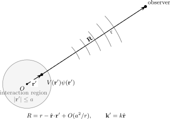
A point $\mathbf r'$ inside a localized interaction region contributes an outgoing wave over the distance $R=|\mathbf r-\mathbf r'|$. In the far zone, $R=r-\hat{\mathbf r}\cdot\mathbf r'+O(a^2/r)$, so the source-dependent phase becomes $e^{-i\mathbf k'\cdot\mathbf r'}$ with $\mathbf k'=k\hat{\mathbf r}$.

From a Distributed Source to the Amplitude

For a local short-range potential, the outgoing Lippmann–Schwinger equation in the unit-incident-amplitude convention is

$$\begin{aligned} \psi_{\mathbf k}^{(+)}(\mathbf r) ={}& e^{i\mathbf k\cdot\mathbf r} \\ &+ \int d^3r'\, G_0^{(+)} (\mathbf r,\mathbf r';E) \\ &\qquad\times V(\mathbf r') \psi_{\mathbf k}^{(+)}(\mathbf r'). \end{aligned}$$

The product

$$s_{\mathbf k}(\mathbf r') = V(\mathbf r') \psi_{\mathbf k}^{(+)}(\mathbf r')$$

is an effective source. Every point in the interaction region radiates through the same outgoing kernel, and the measured far field is their coherent sum.

Using the factorized kernel gives

$$\psi_{\mathbf k}^{(+)}(\mathbf r) \sim e^{i\mathbf k\cdot\mathbf r} + f(\mathbf k',\mathbf k) \frac{e^{ikr}}{r},$$

where

$$\begin{aligned} f(\mathbf k',\mathbf k) ={}& -\frac{\mu}{2\pi\hbar^2} \int d^3r'\, e^{-i\mathbf k'\cdot\mathbf r'} \\ &\qquad\times V(\mathbf r') \psi_{\mathbf k}^{(+)}(\mathbf r'), \end{aligned}$$

and

$$|\mathbf k'|=|\mathbf k|=k.$$

This amplitude formula is exact under the stated potential-scattering and short-range assumptions. The outgoing Green function does not make a Born approximation. That approximation begins only when the exact wave inside the source is replaced by the incident plane wave.

The far-field step also explains why the observable amplitude is on shell. The Green function contains every intermediate wave vector $\mathbf q$ in its Fourier integral, but a distant free outgoing wave at fixed energy has magnitude $k$. The detector direction chooses only $\hat{\mathbf r}$.

With unit incident amplitude,

$$\frac{d\sigma}{d\Omega} = |f(\mathbf k',\mathbf k)|^2.$$

The flux derivation and its interference subtleties belong to Probability Current and Flux.

Relation to the T-matrix

For the delta-normalized wave-number states in the convention ledger,

$$T(E+i0) \lvert\mathbf k\rangle = V \lvert\psi_{\mathbf k}^{(+)}\rangle,$$

where the state on the right now carries delta normalization. Converting from that state to the unit-amplitude coordinate solution gives

$$\begin{aligned} f(\mathbf k',\mathbf k) ={}& -\frac{4\pi^2\mu}{\hbar^2} \\ &\times \langle\mathbf k'\lvert T(E+i0) \rvert\mathbf k\rangle. \end{aligned}$$

The factor differs in other state normalizations. T-Matrix owns the full normalization ledger, shell structure, unitarity relation, and operator identities.

Free and Full Green Functions

The kernel used to radiate the source in the Lippmann–Schwinger equation is the free Green function. The full outgoing Green function is

$$\begin{aligned} G^{(+)}(E) &= \frac{1}{E-H+i0}, \\ H &= H_0+V. \end{aligned}$$

The resolvent identities give

$$\begin{aligned} G^{(+)} &= G_0^{(+)} + G_0^{(+)}V G^{(+)}, \\ &= G_0^{(+)} + G_0^{(+)}T^{(+)}G_0^{(+)}. \end{aligned}$$

These formulas assign distinct jobs:

• $G_0^{(+)}$ propagates between interactions with the chosen free radiation condition;
• $T^{(+)}$ contains one or arbitrarily many interactions;
• $G^{(+)}$ is the complete response of the interacting Hamiltonian.

Taking a distant endpoint of an external $G_0^{(+)}$ factor produces the same far-field on-shell projection derived above. Poles and cuts of the full resolvent then encode bound states, thresholds, and resonances; their canonical treatment is Bound States and Scattering Poles.

Partial-Wave Form

For a central problem, define

$$r_{\min}=\min(r,r'), \qquad r_{\max}=\max(r,r'),$$

and let $\gamma$ be the angle between $\mathbf r$ and $\mathbf r'$. The addition theorem gives

$$\begin{aligned} G_0^{(+)} (\mathbf r,\mathbf r';E) ={}& -\frac{i\mu k}{2\pi\hbar^2} \\ &\times \sum_{\ell=0}^{\infty} (2\ell+1) \\ &\times j_\ell(kr_{\min}) \\ &\times h_\ell^{(1)}(kr_{\max}) P_\ell(\cos\gamma). \end{aligned}$$

Regular spherical Bessel functions appear at the smaller radius, while the outgoing spherical Hankel function appears at the larger radius. Replacing $h_\ell^{(1)}$ by $h_\ell^{(2)}$ gives the incoming kernel. This is the Green-function version of choosing an outgoing radial solution in each angular-momentum channel; see Partial-Wave Expansion.

Dimension Changes the Far Field

The inverse of the same free Schrödinger operator has dimension-dependent asymptotics. For $E=\hbar^2k^2/(2\mu)$:

Dimension	Outgoing free kernel	Far-field decay
one	$-\dfrac{i\mu}{\hbar^2k}e^{ik\lvert x-x'\rvert}$	constant magnitude
two	$-\dfrac{i\mu}{2\hbar^2}H_0^{(1)}(kR)$	$R^{-1/2}$
three	$-\dfrac{\mu}{2\pi\hbar^2}\dfrac{e^{ikR}}{R}$	$R^{-1}$

Cross-section dimensions and amplitude conventions change with the spatial dimension. A three-dimensional formula for $d\sigma/d\Omega$ cannot be carried into a one- or two-dimensional calculation by changing only the measure.

Finite Broadening Is Not the Limit

Numerical calculations often replace $i0$ by a finite $i\eta$, with $\eta\gt0$. Define

$$k_\eta = \frac{ \sqrt{2\mu(E+i\eta)} }{ \hbar },$$

choosing the branch with positive imaginary part. For small $\eta$,

$$k_\eta = k + i\frac{\eta}{\hbar v} + O\left( k\frac{\eta^2}{E^2} \right), \qquad v=\frac{\hbar k}{\mu}.$$

The nominally outgoing wave then behaves as

$$e^{ik_\eta R} \simeq e^{ikR} e^{-R/\ell_\eta}, \qquad \ell_\eta=\frac{\hbar v}{\eta}.$$

A finite regulator therefore adds an absorption length. It can smooth a discrete numerical spectrum and suppress reflections, but it is not the exact radiation condition. A convergence study must compare $\eta$, the energy resolution, the box size, and the distance over which the outgoing wave is measured.

The kernel is also singular at $\mathbf r=\mathbf r'$. Integral-equation solvers should treat that known singularity analytically or with a quadrature designed for it rather than sampling it as an ordinary smooth function.

Limits of the Free-Kernel Argument

Threshold

At $k=0$, the oscillatory Sommerfeld condition degenerates and the distinction between $e^{ikr}$ and $e^{-ikr}$ disappears at leading order. Zero-energy resonances and large scattering lengths require a separate threshold limit. The limits $r\to\infty$ and $k\to0$ need not commute.

Long-range interactions

For an unscreened Coulomb potential, the exact asymptotic state contains a logarithmic phase and is not a plane wave plus a short-range spherical wave. One should use Coulomb-distorted reference states or a Coulomb Green function. See Coulomb Scattering.

Several channels

In a multichannel problem, each open channel $\alpha$ has its own real wave number $k_\alpha$ and outgoing kernel. A closed channel has $k_\alpha=i\kappa_\alpha$ and decays exponentially instead of carrying asymptotic flux. The Green function becomes a matrix in channel space, and velocity factors enter observable cross sections.

Nonlocal or absorptive interactions

For a nonlocal interaction, the source is

$$s(\mathbf r') = \int d^3x\, V(\mathbf r',\mathbf x) \psi(\mathbf x),$$

but the free kernel still carries that source to the far field. If $V$ is complex, the outgoing prescription remains meaningful, although elastic probability need not be conserved because the effective interaction represents loss into omitted channels.

QFT Propagator Bridge

The nonrelativistic fixed-energy kernel has momentum denominator

$$\frac{1}{ E-\mathbf p^2/(2\mu)+i0 }.$$

A relativistic scalar Feynman propagator, in a common convention, has

$$D_F(p) = \frac{i}{ p^2-m^2+i0 }.$$

Both formulas use analytic boundary prescriptions, but they are not the same object:

• $G_0^{(+)}(E)$ is a one-particle resolvent boundary value at fixed energy and selects outgoing spatial radiation;
• $D_F$ is a spacetime vacuum correlation function whose pole prescription implements time ordering;
• a retarded relativistic propagator uses a different placement of the energy poles;
• LSZ reduction extracts scattering amplitudes from pole residues of time-ordered correlation functions rather than from a potential source integral.

The propagator of a nonrelativistic quantum field,

$$\frac{i}{ p^0-\mathbf p^2/(2m)+i0 },$$

is algebraically closer to the resolvent, but its energy is integrated in diagrams and its normalization follows field-theory conventions. The careful translation is developed in Green Functions and Bridge to QFT Scattering.

Common Mistakes

• Treating $(E-H_0)^{-1}$ as an ordinary inverse at a continuum energy.
• Dropping $i0$ before it has selected a boundary value.
• Calling $+i0$ outgoing without stating the time and Fourier conventions.
• Applying the Sommerfeld condition to the total incident-plus-scattered wave.
• Using $r\gg a$ but ignoring the stronger phase condition $ka^2/r\ll1$.
• Replacing the exact source wave by a plane wave without naming the Born approximation.
• Mixing unit-amplitude coordinate waves with delta-normalized $T$-matrix states.
• Assuming $G_0^{(+)}$ is Hermitian rather than recognizing that its adjoint is $G_0^{(-)}$.
• Interpreting a finite $\eta$ as a harmless infinitesimal even when its absorption length is comparable to the numerical domain.
• Using a free short-range kernel for unscreened Coulomb asymptotics.
• Taking the three-dimensional $1/r$ decay and cross-section formula into another spatial dimension.
• Equating an outgoing Schrödinger resolvent with a Feynman propagator.

Cross-Links

• Energy Green Function
• Resolvent Operator
• Retarded and Advanced Green Functions
• Scattering States and Boundary Conditions
• Lippmann–Schwinger Equation
• Scattering Amplitude
• T-Matrix
• Born Series
• Probability Current and Flux
• Partial-Wave Expansion
• Coulomb Scattering
• Scattering Convention Dictionary
• Green Functions

References

1. B. A. Lippmann and J. Schwinger, “Variational principles for scattering processes. I”, Physical Review 79, 469–480 (1950).
2. J. R. Taylor, Scattering Theory: The Quantum Theory of Nonrelativistic Collisions, Dover (2006).
3. R. G. Newton, Scattering Theory of Waves and Particles, 2nd ed., Dover (2002).
4. C. J. Joachain, Quantum Collision Theory, 3rd ed., North-Holland (1983).
5. E. N. Economou, Green’s Functions in Quantum Physics, 3rd ed., Springer (2006).
6. M. Reed and B. Simon, Methods of Modern Mathematical Physics, Vol. III: Scattering Theory, Academic Press (1979).
7. NIST Digital Library of Mathematical Functions, §10.17, “Asymptotic Expansions for Large Argument” and §10.73, “Physical Applications”.

Exercises

Read the direction from the current

For

$$\psi_\pm(\mathbf r) = A \frac{e^{\pm ikr}}{r},$$

compute the leading radial current and identify which sign is outgoing for time dependence $e^{-iEt/\hbar}$.

Solution

The radial current is

$$j_r = \frac{\hbar}{2\mu i} \left( \psi_\pm^*\partial_r\psi_\pm - \psi_\pm\partial_r\psi_\pm^* \right).$$

The derivative of $1/r$ is real and cancels between the two terms. The phase derivative gives

$$j_r = \pm \frac{\hbar k}{\mu} \frac{|A|^2}{r^2}.$$

The plus sign carries positive radial flux and is outgoing. The minus sign carries negative radial flux and is incoming.

Control the far-field approximation

Let $|\mathbf r'|\le a$ and $\mathbf r=r\hat{\mathbf r}$. Expand $|\mathbf r-\mathbf r'|$ through order $1/r$ and identify the two dimensionless errors in replacing the outgoing kernel by its factorized far-field form.

Solution

Write

$$\begin{aligned} |\mathbf r-\mathbf r'| &= r \left[ 1 - \frac{ 2\hat{\mathbf r}\cdot\mathbf r' }{ r } + \frac{r'^2}{r^2} \right]^{1/2}. \end{aligned}$$

Expanding the square root gives

$$\begin{aligned} |\mathbf r-\mathbf r'| ={}& r-\hat{\mathbf r}\cdot\mathbf r' \\ &+ \frac{ r'^2- (\hat{\mathbf r}\cdot\mathbf r')^2 }{ 2r } + O\left(\frac{a^3}{r^2}\right). \end{aligned}$$

Replacing $1/R$ by $1/r$ has relative error $O(a/r)$. Dropping the quadratic term from $kR$ has phase error $O(ka^2/r)$. Both must be small.

Verify the resolvent jump in coordinate space

Use the explicit three-dimensional kernels to compute

$$G_0^{(+)}(R;E)-G_0^{(-)}(R;E),$$

and verify that it equals

$$-2\pi i \langle\mathbf r\vert \delta(E-H_0) \rvert\mathbf r'\rangle.$$

Solution

The explicit kernels give

$$\begin{aligned} G_0^{(+)}-G_0^{(-)} &= -\frac{\mu}{2\pi\hbar^2R} \left( e^{ikR}-e^{-ikR} \right) \\ &= -\frac{i\mu}{\pi\hbar^2} \frac{\sin(kR)}{R}. \end{aligned}$$

In the wave-number basis,

$$\begin{aligned} \langle\mathbf r\vert \delta(E-H_0) \rvert\mathbf r'\rangle ={}& \int\frac{d^3q}{(2\pi)^3} e^{i\mathbf q\cdot\mathbf R} \\ &\times \delta \left( E-\frac{\hbar^2q^2}{2\mu} \right). \end{aligned}$$

The radial delta function fixes $q=k$, yielding

$$\langle\mathbf r\vert \delta(E-H_0) \rvert\mathbf r'\rangle = \frac{\mu}{2\pi^2\hbar^2} \frac{\sin(kR)}{R}.$$

Multiplication by $-2\pi i$ reproduces the kernel difference.

Interpret a finite regulator

For $E\gt0$, replace $i0$ by $i\eta$ with $\eta\gt0$. Show that the outgoing wave is attenuated over the length $\ell_\eta=\hbar v/\eta$ to leading order.

Solution

The complex wave number is

$$k_\eta = \sqrt{ k^2+ i\frac{2\mu\eta}{\hbar^2} }.$$

Expanding the square root gives

$$k_\eta = k+ i\frac{\mu\eta}{\hbar^2k} + O\left( k\frac{\eta^2}{E^2} \right).$$

Since $v=\hbar k/\mu$,

$$\frac{\mu\eta}{\hbar^2k} = \frac{\eta}{\hbar v}.$$

Therefore

$$e^{ik_\eta R} \simeq e^{ikR} \exp\left( -\frac{\eta R}{\hbar v} \right) = e^{ikR}e^{-R/\ell_\eta},$$

with $\ell_\eta=\hbar v/\eta$.

Translate the amplitude normalization

Let $\psi_{\mathbf k}^{(+)}(\mathbf r)$ have unit incident amplitude. The corresponding delta-normalized state has coordinate wavefunction

$$\langle\mathbf r\vert \psi_{\mathbf k}^{(+)} \rangle_{\delta} = \frac{1}{(2\pi)^{3/2}} \psi_{\mathbf k}^{(+)}(\mathbf r).$$

Show that

$$f = -\frac{\mu}{2\pi\hbar^2} \int d^3r\, e^{-i\mathbf k'\cdot\mathbf r} V(\mathbf r) \psi_{\mathbf k}^{(+)}(\mathbf r)$$

becomes

$$f = -\frac{4\pi^2\mu}{\hbar^2} \langle\mathbf k'\vert T(E+i0) \vert\mathbf k\rangle$$

in the delta-normalized basis.

Solution

Using

$$\langle\mathbf r\vert\mathbf k'\rangle = \frac{ e^{i\mathbf k'\cdot\mathbf r} }{ (2\pi)^{3/2} },$$

and

$$T(E+i0)\lvert\mathbf k\rangle = V\lvert\psi_{\mathbf k}^{(+)}\rangle_\delta,$$

one finds

$$\begin{aligned} \langle\mathbf k'\vert T \vert\mathbf k\rangle ={}& \frac{1}{(2\pi)^3} \int d^3r\, e^{-i\mathbf k'\cdot\mathbf r} \\ &\qquad\times V(\mathbf r) \psi_{\mathbf k}^{(+)}(\mathbf r). \end{aligned}$$

The integral is therefore $(2\pi)^3$ times the $T$-matrix element. Since

$$\frac{\mu}{2\pi\hbar^2} (2\pi)^3 = \frac{4\pi^2\mu}{\hbar^2},$$

the stated relation follows.