Scattering States and Boundary Conditions

A positive-energy solution of the stationary Schrödinger equation is not yet a fully specified scattering state. One must also say what is incident, what is allowed to arrive from infinity, and what is allowed to radiate outward. Those asymptotic data play the role that endpoint boundary conditions play for a bound-state problem.

For a short-range interaction in three dimensions, the physical state generated by an incident plane wave has the schematic form

$$\begin{gathered} \text{incident free wave} \\ {}+\; \text{outgoing scattered wave}. \end{gathered}$$

The word outgoing is a mathematical condition, not a picture added after solving the equation. It selects one boundary value of the continuum resolvent and makes the scattering problem well posed.

This page is the canonical home for asymptotic scattering boundary conditions and continuum-state normalization. Lippmann–Schwinger Equation owns the exact state equation, Energy Green Function owns general coordinate-kernel normalization, Green Function for Scattering owns the outgoing-kernel and far-field derivation, and Scattering Amplitude owns the amplitude convention.

Why the Eigenvalue Equation Is Not Enough

Consider the one-channel relative-motion Hamiltonian

$$H = H_0+V, \qquad H_0 = \frac{\mathbf p^2}{2\mu},$$

where $\mu$ is the reduced mass. At energy

$$E = \frac{\hbar^2k^2}{2\mu}, \qquad k\gt0,$$

a stationary state satisfies

$$(H-E)\psi=0.$$

Outside the range of a sufficiently short-range potential, this becomes the Helmholtz equation

$$(\nabla^2+k^2)\psi=0.$$

That equation admits plane waves, incoming spherical waves, outgoing spherical waves, standing waves, and arbitrary superpositions. Regularity near the interaction region does not by itself decide which combination represents the experiment.

A scattering problem therefore specifies two kinds of information:

1. incident data: the free channel prepared in the distant past;
2. radiation data: no additional scattered radiation is allowed to arrive from infinity.

Together with the differential equation, those data select the physical solution.

Free Asymptotic States

For the simplest free relative motion, generalized momentum eigenstates obey

$$H_0\lvert\mathbf k\rangle = \frac{\hbar^2k^2}{2\mu} \lvert\mathbf k\rangle.$$

With the convention

$$\langle\mathbf r\vert\mathbf k\rangle = \frac{e^{i\mathbf k\cdot\mathbf r}}{(2\pi)^{3/2}},$$

their normalization is

$$\langle\mathbf k\vert\mathbf k'\rangle = \delta^{(3)}(\mathbf k-\mathbf k').$$

These kets are generalized eigenvectors, not square-integrable Hilbert-space vectors. They are useful because a sharply defined incident momentum makes energy conservation and angular dependence transparent.

In a multichannel problem, the label $\alpha$ supplements momentum with every asymptotic internal quantum number:

$$\lvert\phi_\alpha\rangle = \lvert\mathbf k_\alpha,\nu_\alpha\rangle.$$

The free channel Hamiltonian fixes the threshold and channel speed. Closed channels can influence the interaction region, but only open channels carry asymptotic flux to infinity.

The Physical Outgoing State

Let the incident momentum be $\mathbf k=k\hat{\mathbf k}$. For a short-range potential, the state denoted by $\psi_{\mathbf k}^{(+)}$ has asymptotic form

$$\begin{aligned} \psi_{\mathbf k}^{(+)}(\mathbf r) ={}& e^{i\mathbf k\cdot\mathbf r} \\ &+ f(\hat{\mathbf r}\leftarrow\hat{\mathbf k};k) \frac{e^{ikr}}{r} + o(r^{-1}). \end{aligned}$$

The plane wave specifies the incident channel. The spherical term is the field generated by the interaction, and its radial phase is outgoing for the time convention

$$\Psi(\mathbf r,t) = e^{-iEt/\hbar} \psi(\mathbf r).$$

Indeed, a constant phase of

$$e^{i(kr-Et/\hbar)}$$

moves toward increasing $r$. The phase of $e^{-i(kr+Et/\hbar)}$ moves toward decreasing $r$ and is incoming.

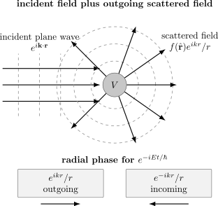
With time dependence $e^{-iEt/\hbar}$, the factor $e^{ikr}/r$ carries radial phase away from the target. The incident plane wave is part of the specified preparation; the radiation condition applies to the scattered remainder.

The superscript $(+)$ labels the outgoing boundary prescription. It does not mean positive energy, positive momentum, or a positive-frequency projection.

The Sommerfeld Radiation Condition

Write the total state as

$$\psi = \phi_{\mathrm{in}} + \psi_{\mathrm{sc}},$$

where $\phi_{\mathrm{in}}$ is the specified free incident solution. In three dimensions, the outgoing Sommerfeld condition is

$$\lim_{r\to\infty} r \left( \frac{\partial}{\partial r}-ik \right) \psi_{\mathrm{sc}}(\mathbf r) = 0$$

uniformly in direction under the usual short-range assumptions. An incoming scattered field obeys the opposite condition:

$$\lim_{r\to\infty} r \left( \frac{\partial}{\partial r}+ik \right) \psi_{\mathrm{sc}}(\mathbf r) = 0.$$

For

$$\psi_{\mathrm{sc}} = f(\hat{\mathbf r}) \frac{e^{ikr}}{r},$$

the outgoing operator gives

$$\left( \partial_r-ik \right) \psi_{\mathrm{sc}} = - f(\hat{\mathbf r}) \frac{e^{ikr}}{r^2},$$

so multiplying by $r$ makes the result vanish at infinity.

The condition must be imposed on $\psi_{\mathrm{sc}}$, not on the total state. A plane wave extends through all space and does not satisfy a purely outgoing spherical radiation condition. Its role is to supply the incident field against which the scattered field is defined.

For appropriate short-range problems, the incident field plus the outgoing radiation condition gives a unique solution. Physically, it excludes an arbitrary source of incoming spherical radiation located at infinity.

The i0 Prescription

The same boundary choice appears in operator language. The free resolvent boundary values are

$$G_0^{(\pm)}(E) = \lim_{\epsilon\to0^+} \frac{1}{E-H_0\pm i\epsilon}.$$

For the time dependence $e^{-iEt/\hbar}$,

$$G_0^{(+)} \quad\longleftrightarrow\quad \text{outgoing},$$

while $G_0^{(-)}$ is incoming. In three dimensions,

$$\begin{aligned} \langle\mathbf r\vert G_0^{(+)}(E) \vert\mathbf r'\rangle ={}& -\frac{\mu}{2\pi\hbar^2} \\ &\times \frac{ e^{ik\lvert\mathbf r-\mathbf r'\rvert} }{ \lvert\mathbf r-\mathbf r'\rvert }. \end{aligned}$$

The sign is not an arbitrary mnemonic. The scalar distribution identity

$$\frac{1}{x\pm i0} = \operatorname{PV}\frac{1}{x} \mp i\pi\delta(x)$$

selects a boundary value across the continuous spectrum. Fourier transformation turns that analytic choice into outgoing or incoming spatial behavior.

The Lippmann–Schwinger equation then reads

$$\lvert\psi_\alpha^{(\pm)}\rangle = \lvert\phi_\alpha\rangle + G_0^{(\pm)}(E) V \lvert\psi_\alpha^{(\pm)}\rangle.$$

The finite $\epsilon$ sometimes used in numerics adds artificial broadening. The exact notation $\pm i0$ means a distributional limit; it is not a small physical absorption coefficient.

Incoming States and Final Channels

The state $\psi_\alpha^{(-)}$ has an incoming scattered-wave condition. In the same short-range one-channel notation,

$$\begin{aligned} \psi_{\mathbf k}^{(-)}(\mathbf r) ={}& e^{i\mathbf k\cdot\mathbf r} \\ &+ f^{(-)}(\hat{\mathbf r}\leftarrow\hat{\mathbf k};k) \, \\ &\quad\times \frac{e^{-ikr}}{r} + o(r^{-1}). \end{aligned}$$

This solution is not usually the state prepared by firing one plane-wave beam at a target. Its central role is to represent a specified final channel in transition amplitudes.

The temporal meaning is encoded by the Møller wave operators:

$$\Omega^{(\pm)} = \operatorname*{s-lim}_{t\to\mp\infty} e^{iHt/\hbar} e^{-iH_0t/\hbar}.$$

When these limits exist,

$$\lvert\psi_\alpha^{(\pm)}\rangle = \Omega^{(\pm)} \lvert\phi_\alpha\rangle.$$

Thus $\psi_\alpha^{(+)}$ approaches the chosen free channel in the distant past, whereas $\psi_\beta^{(-)}$ approaches the chosen free channel in the distant future. The scattering operator is

$$S = \Omega^{(-)\dagger} \Omega^{(+)},$$

and its channel matrix element can be written

$$S_{\beta\alpha} = \langle\psi_\beta^{(-)} \vert \psi_\alpha^{(+)}\rangle.$$

This is why both signs appear in a physical calculation: the plus state represents the prepared incoming channel, and the minus state tests a selected outgoing channel.

S-Matrix develops the resulting operator map, its energy-shell channel matrices, and the completeness assumptions behind unitarity.

Partial Waves and Radial Direction

For a central short-range potential, each angular-momentum channel has asymptotic reduced radial function

$$\begin{aligned} u_\ell(k,r) \sim \frac{1}{2i} \Big[ & S_\ell(k) e^{i(kr-\ell\pi/2)} \\ &- e^{-i(kr-\ell\pi/2)} \Big]. \end{aligned}$$

The second exponential is incoming, while the first is outgoing. With no interaction, $S_\ell=1$ and the expression becomes the regular standing wave

$$u_\ell(k,r) \sim \sin(kr-\ell\pi/2).$$

This does not contradict the plane-wave-plus-outgoing-wave form. A plane wave itself contains both incoming and outgoing spherical components when expanded in partial waves. The interaction changes only the outgoing coefficient relative to the specified incident content. Partial-Wave Expansion and Phase Shifts develop this decomposition.

For one elastic channel and a real potential,

$$S_\ell=e^{2i\delta_\ell}, \qquad \lvert S_\ell\rvert=1.$$

When inelastic channels are open, an individual elastic element can have magnitude below one because outgoing flux is shared among channels.

Momentum and Energy Normalization

Continuum labels carry Jacobians. Starting from

$$\langle\mathbf k\vert\mathbf k'\rangle = \delta^{(3)}(\mathbf k-\mathbf k'),$$

the spherical-coordinate identity is

$$\delta^{(3)}(\mathbf k-\mathbf k') = \frac{1}{k^2} \delta(k-k') \delta^{(2)} (\hat{\mathbf k}-\hat{\mathbf k}').$$

Define radial-momentum states by

$$\lvert k,\hat{\mathbf k}\rangle \equiv k\lvert\mathbf k\rangle.$$

They obey

$$\begin{aligned} \langle k,\hat{\mathbf k} \vert k',\hat{\mathbf k}'\rangle ={}& \delta(k-k') \\ &\times \delta^{(2)} (\hat{\mathbf k}-\hat{\mathbf k}'). \end{aligned}$$

Because

$$\frac{dE}{dk} = \frac{\hbar^2k}{\mu},$$

energy-normalized states are

$$\begin{aligned} \lvert E,\hat{\mathbf k}\rangle &= \sqrt{\frac{dk}{dE}}\, \lvert k,\hat{\mathbf k}\rangle \\ &= \sqrt{\frac{\mu k}{\hbar^2}}\, \lvert\mathbf k\rangle. \end{aligned}$$

Their inner product is

$$\begin{aligned} \langle E,\hat{\mathbf k} \vert E',\hat{\mathbf k}'\rangle ={}& \delta(E-E') \\ &\times \delta^{(2)} (\hat{\mathbf k}-\hat{\mathbf k}'). \end{aligned}$$

This normalization is convenient because energy-conserving $S$-matrix elements carry a simple $\delta(E-E')$. Momentum normalization, energy normalization, box normalization, and unit-flux normalization distribute factors of $k$, velocity, $2\pi$, and $\hbar$ differently. They are equivalent only when every state, amplitude, delta function, and phase-space measure is transformed consistently.

For a plane wave $Ae^{ikz}$,

$$j_z = \frac{\hbar k}{\mu} \lvert A\rvert^2 = v\lvert A\rvert^2.$$

Unit-flux channel functions therefore contain a factor proportional to $v^{-1/2}$. This velocity factor becomes essential when incident and outgoing channels have different masses, thresholds, or momenta.

Wave Packets Versus Plane Waves

Plane waves provide exact energy resolution and stationary incident flux, but they are not localized and cannot describe a finite preparation by themselves. A normalizable incoming packet is a superposition

$$\lvert\Psi^{(+)}\rangle = \int d^3k\, a(\mathbf k) \lvert\psi_{\mathbf k}^{(+)}\rangle,$$

with

$$\int d^3k\, \lvert a(\mathbf k)\rvert^2 = 1$$

for the momentum normalization used above.

If $a(\mathbf k)$ is concentrated around $\mathbf k_0$, then in the distant past the packet is localized far from the target and moves inward with group velocity

$$\mathbf v_g = \frac{\hbar\mathbf k_0}{\mu}.$$

After the collision, the state separates into outgoing packets in the available channels. The stationary amplitude is recovered when the packet is narrow in momentum and the detector probes distances large compared with the interaction range and packet scales.

The plane-wave formalism is therefore not a claim that physical beams fill all space. It is a distributional basis used to compute how normalizable packets scatter. Gaussian Wave Packets supplies the canonical localized free state, while What Is a Scattering Experiment? connects such preparations to finite beams and detectors.

Numerical Boundary Conditions

An infinite domain must be represented somehow in a finite calculation.

• radial matching: integrate through the interaction region and match to known incoming and outgoing free or Coulomb functions at a sufficiently large radius;
• logarithmic derivative: propagate $u_\ell'/u_\ell$ and extract $S_\ell$ without fixing an arbitrary overall normalization;
• absorbing layer or complex absorber: damp outgoing waves before they reach the numerical boundary;
• exterior complex scaling: rotate the asymptotic coordinate so outgoing resonance solutions become decaying;
• large box: discretize the continuum and infer scattering information from level shifts or matching.

An absorber is a computational device, not the exact meaning of $+i0$. It must be tested for spurious reflection and dependence on absorber strength and location. A hard wall produces standing waves and therefore changes the scattering boundary condition unless a finite-volume method explicitly accounts for it.

Rigorous Caveats

The familiar formulas hide assumptions.

Short-range interactions

The plane-wave-plus-$e^{ikr}/r$ asymptotic form is valid for appropriate short-range potentials. An unscreened Coulomb tail produces a logarithmic phase and requires distorted asymptotic states. Coulomb Scattering owns that case.

Thresholds

At $k=0$, the oscillatory Sommerfeld condition degenerates. Zero-energy resonances, half-bound states, and divergent scattering lengths require separate threshold analysis.

Bound states

Møller operators map free states into the absolutely continuous scattering subspace. Normalizable bound states are not generated from incident free packets and must be included separately in a completeness relation.

Existence and completeness

The limits defining $\Omega^{(\pm)}$ need not exist for every interaction. Even when they exist, asymptotic completeness

$$\operatorname{Ran}\Omega^{(+)} = \operatorname{Ran}\Omega^{(-)} = \mathcal H_{\mathrm{ac}}(H)$$

is a theorem requiring hypotheses, not a formal identity. Long-range forces, many-body breakup, singular interactions, and embedded spectral structure can demand modified constructions.

Resonance states

A resonance is often characterized by a purely outgoing condition at complex energy with no incident plane wave. Such a Gamow-type state is not the same object as a physical real-energy $\psi^{(+)}$, which contains specified incident data.

Common Mistakes

• Treating $(+)$ and $(-)$ as signs of energy or momentum rather than boundary prescriptions.
• Imposing the Sommerfeld condition on the total plane-wave-plus-scattered state instead of the scattered remainder.
• Calling $e^{-ikr}/r$ outgoing while using the time convention $e^{-iEt/\hbar}$.
• Replacing $+i0$ by a finite numerical broadening without checking the limiting behavior.
• Normalizing a plane wave to one over all space as though it were a bound state.
• Changing from $k$ normalization to $E$ normalization without the Jacobian $\sqrt{dk/dE}$.
• Assuming the ordinary short-range asymptotic form remains valid for an unscreened Coulomb potential.
• Interpreting a finite hard-wall calculation as an outgoing scattering problem without a matching or finite-volume prescription.
• Confusing a physical incident-plus-outgoing state with a purely outgoing resonance state.

Cross-Links

• Scattering Theory
• What Is a Scattering Experiment?
• Normalization Conventions
• Scattering Amplitude
• Lippmann–Schwinger Equation
• Energy Green Function
• Partial-Wave Expansion
• Phase Shifts
• Coulomb Scattering
• Bound States and Scattering Poles
• Resonances

References

• J. R. Taylor, Scattering Theory: The Quantum Theory of Nonrelativistic Collisions, Wiley, 1972, Chapters 2–4.
• R. G. Newton, Scattering Theory of Waves and Particles, 2nd ed., Springer, 1982, Chapters 5–8.
• C. J. Joachain, Quantum Collision Theory, North-Holland, 1975, Chapters 2–4.
• M. Reed and B. Simon, Methods of Modern Mathematical Physics, Vol. III: Scattering Theory, Academic Press, 1979.
• D. R. Yafaev, Mathematical Scattering Theory: General Theory, American Mathematical Society, 1992.
• J. J. Sakurai and J. Napolitano, Modern Quantum Mechanics, 3rd ed., Cambridge University Press, 2020.
• B. A. Lippmann and J. Schwinger, “Variational Principles for Scattering Processes. I,” Physical Review 79, 469–480 (1950), DOI: 10.1103/PhysRev.79.469.

Exercises

1. Radial phase direction

Using the time dependence $e^{-iEt/\hbar}$, show that $e^{ikr}/r$ is outgoing and $e^{-ikr}/r$ is incoming.

Solution

The outgoing phase is

$$\Phi_+(r,t) = kr-\frac{Et}{\hbar}.$$

Holding it constant gives

$$\frac{dr}{dt} = \frac{E}{\hbar k} \gt0.$$

For the other sign,

$$\Phi_-(r,t) = -kr-\frac{Et}{\hbar},$$

so

$$\frac{dr}{dt} = -\frac{E}{\hbar k} \lt0.$$

The $1/r$ factor changes the amplitude, not the direction of phase propagation.

2. Test the radiation condition

Let $\psi_{\mathrm{sc}}=f(\hat{\mathbf r})e^{ikr}/r$. Verify the outgoing Sommerfeld condition and show that the incoming spherical wave fails it.

Solution

For the outgoing wave,

$$\left( \partial_r-ik \right) \frac{f e^{ikr}}{r} = - \frac{f e^{ikr}}{r^2}.$$

Multiplication by $r$ leaves a term of order $r^{-1}$, which vanishes. For the incoming wave,

$$\begin{aligned} \left( \partial_r-ik \right) \frac{f e^{-ikr}}{r} ={}& -\frac{f e^{-ikr}}{r^2} \\ &- \frac{2ikf e^{-ikr}}{r}. \end{aligned}$$

After multiplication by $r$, the second term does not vanish. It instead satisfies the radiation condition with $\partial_r+ik$.

3. Derive energy normalization

Starting from $\langle k,\hat{\mathbf k}\vert k',\hat{\mathbf k}'\rangle=\delta(k-k')\delta^{(2)}(\hat{\mathbf k}-\hat{\mathbf k}')$, derive the factor relating $\lvert E,\hat{\mathbf k}\rangle$ to $\lvert k,\hat{\mathbf k}\rangle$.

Solution

For $E=\hbar^2k^2/(2\mu)$,

$$\frac{dk}{dE} = \frac{\mu}{\hbar^2k}.$$

The transformed state must be

$$\lvert E,\hat{\mathbf k}\rangle = \sqrt{\frac{dk}{dE}}\, \lvert k,\hat{\mathbf k}\rangle.$$

Then

$$\begin{aligned} \langle E,\hat{\mathbf k} \vert E',\hat{\mathbf k}'\rangle ={}& \delta(E-E') \\ &\times \delta^{(2)} (\hat{\mathbf k}-\hat{\mathbf k}'). \end{aligned}$$

The square root is required because the Jacobian appears once from the bra and once from the ket.

4. Free partial-wave limit

Set $S_\ell=1$ in the asymptotic radial expression and recover the regular free standing wave. Explain why this does not add an independently prepared incoming spherical beam.

Solution

With $x=kr-\ell\pi/2$,

$$\frac{1}{2i} \left( e^{ix}-e^{-ix} \right) = \sin x.$$

This is the large-$r$ behavior of the regular free spherical Bessel solution. The incoming radial component is already part of the partial-wave decomposition of the specified incident plane wave. The scattering boundary condition forbids an additional incoming scattered field; it does not remove the incoming pieces needed to reconstruct the plane wave.

5. Packet interpretation

Why does a square-integrable packet resolve the apparent tension between a physical finite beam and the non-normalizable plane waves used in stationary scattering theory?

Solution

A packet superposes continuum states with a square-integrable weight:

$$\lvert\Psi^{(+)}\rangle = \int d^3k\, a(\mathbf k) \lvert\psi_{\mathbf k}^{(+)}\rangle.$$

The delta normalization of the stationary states gives

$$\langle\Psi^{(+)} \vert \Psi^{(+)}\rangle = \int d^3k\, \lvert a(\mathbf k)\rvert^2 = 1.$$

The packet is localized and has finite momentum spread. Plane-wave amplitudes are the basis coefficients from which its asymptotic outgoing packets are constructed. Sharp-energy cross sections emerge when the packet is narrow enough that the amplitude and detector response vary little across its support.