Gaussian Wave Packets

A Gaussian wave packet is the canonical localized state for a free particle. It is normalizable, has well-controlled position and momentum uncertainties, and evolves exactly under the free-particle Schrödinger equation. It is the simplest model of a particle that is neither perfectly localized nor completely delocalized.

At $t=0$, a convenient normalized one-dimensional Gaussian packet is

$$\psi(x,0) =\left(\frac{1}{2\pi\sigma_x^2}\right)^{1/4} \exp\left[ -\frac{(x-x_0)^2}{4\sigma_x^2} +\frac{i}{\hbar}p_0(x-x_0) \right].$$

Here $x_0$ is the mean position, $p_0$ is the mean momentum, and $\sigma_x$ is the initial position uncertainty.

The convention matters. In this page, $\sigma_x$ is the standard deviation of the probability density, not the width appearing directly in the wavefunction exponent. A constant global phase has been omitted, and the initial quadratic phase is zero. That last choice makes the packet initially uncorrelated in position and momentum; a Gaussian modulus with a different phase need not have the same uncertainty product.

Two useful dimensionless variables are

$$\xi=\frac{x-x_0}{\sigma_x}, \qquad \tau=\frac{\hbar t}{2m\sigma_x^2}.$$

The characteristic spreading time is therefore

$$t_0=\frac{2m\sigma_x^2}{\hbar},$$

so that $\tau=t/t_0$.

Probability Density

The probability density is

$$\lvert\psi(x,0)\rvert^2 =\frac{1}{\sqrt{2\pi}\sigma_x} \exp\left[-\frac{(x-x_0)^2}{2\sigma_x^2}\right].$$

This is an ordinary Gaussian probability density centered at $x_0$. It satisfies

$$\int_{-\infty}^{\infty}\lvert\psi(x,0)\rvert^2\,dx=1,$$

and

$$\langle x\rangle=x_0, \qquad (\Delta x)_0=\sigma_x.$$

These statements follow from the standard Gaussian moments. With $u=(x-x_0)/\sigma_x$,

$$\int_{-\infty}^{\infty}e^{-u^2/2}\,du =\sqrt{2\pi},$$

the first centered moment vanishes by oddness, and the second centered moment equals $\sigma_x^2$. The wavefunction amplitude falls like a Gaussian with $4\sigma_x^2$ in the denominator of its exponent, while the probability density has $2\sigma_x^2$. Keeping this distinction straight prevents many factor-of-two errors.

Momentum Distribution

Using the unitary Fourier convention

$$\phi(p) =\frac{1}{\sqrt{2\pi\hbar}} \int_{-\infty}^{\infty} e^{-ipx/\hbar}\psi(x,0)\,dx,$$

completing the square gives

\phi(p) =left( \frac{2\sigma_x^2}{\pi\hbar^2} \right)^{1/4} \exp\left[ -\frac{\sigma_x^2(p-p_0)^2}{\hbar^2} -\frac{i}{\hbar}px_0 \right].

The phase $e^{-ipx_0/\hbar}$ records the spatial translation and does not affect the momentum probability density:

$$\lvert\phi(p)\rvert^2 =sqrt{\frac{2\sigma_x^2}{\pi\hbar^2}} \exp\left[ -\frac{2\sigma_x^2(p-p_0)^2}{\hbar^2} \right].$$

It follows that

$$\langle p\rangle_0=p_0, \qquad (\Delta p)_0=\frac{\hbar}{2\sigma_x}.$$

Parseval’s identity gives $\int\lvert\phi(p)\rvert^2dp=1$, consistent with position-space normalization. The packet therefore satisfies

$$(\Delta x)_0(\Delta p)_0=\frac{\hbar}{2}.$$

It saturates the Heisenberg inequality at $t=0$. Narrowing the packet in position necessarily broadens its momentum distribution, and the product stays fixed for this unchirped Gaussian family.

Free Time Evolution

For the free Hamiltonian

$$\hat H=\frac{\hat p^2}{2m},$$

each momentum component evolves by a phase

$$e^{-ip^2t/(2m\hbar)}.$$

The inverse transform therefore gives

$$\psi(x,t) =\frac{1}{\sqrt{2\pi\hbar}} \int_{-\infty}^{\infty}dp\, \phi(p) \exp\left[ \frac{i}{\hbar}px -\frac{i}{\hbar}\frac{p^2}{2m}t \right].$$

The exponent is quadratic in $p$, so the integral is exactly evaluable by completing the square. With $\tau=t/t_0$, the result is

$$\psi(x,t) =\left(\frac{1}{2\pi\sigma_x^2}\right)^{1/4} \frac{1}{\sqrt{1+i\tau}} \exp\left[ -\frac{(x-x_0-p_0t/m)^2} {4\sigma_x^2(1+i\tau)} +\frac{i}{\hbar}p_0(x-x_0) -\frac{i}{\hbar}\frac{p_0^2t}{2m} \right].$$

The square root is chosen continuously so that it equals one at $t=0$. Substituting $t=0$ recovers the initial state, providing a quick phase and factor check.

The probability density is simpler:

$$\lvert\psi(x,t)\rvert^2 =\frac{1}{\sqrt{2\pi}\sigma_x(t)} \exp\left[ -\frac{(x-x_0-p_0t/m)^2}{2\sigma_x^2(t)} \right],$$

where

$$\sigma_x(t) =\sigma_x\sqrt{1+\left(\frac{\hbar t}{2m\sigma_x^2}\right)^2}.$$

The normalization is conserved because the broadened density has height proportional to $1/\sigma_x(t)$. Its moments are

$$\begin{aligned} \langle x\rangle_t &=x_0+\frac{p_0}{m}t, & (\Delta x)_t &=\sigma_x\sqrt{1+\tau^2},\\ \langle p\rangle_t &=p_0, & (\Delta p)_t &=\frac{\hbar}{2\sigma_x}. \end{aligned}$$

The center moves with velocity

$$v_g=\frac{p_0}{m},$$

while the packet spreads.

At $t=t_0$, its position standard deviation has grown to $\sqrt2\,\sigma_x$. At late times,

$$(\Delta x)_t \sim \frac{\Delta p}{m}\lvert t\rvert,$$

which has a direct kinematic interpretation: momentum components with velocity spread $\Delta p/m$ separate ballistically.

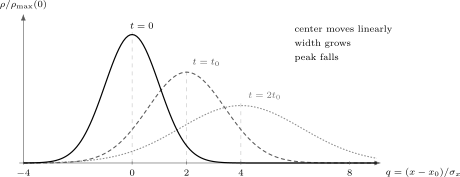
Free evolution at $t=0$, $t=t_0$, and $t=2t_0$ for a representative packet with $p_0t_0/(m\sigma_x)=2$. The center advances linearly while the standard deviation grows from $\sigma_x$ to $\sqrt2\,\sigma_x$ and then $\sqrt5\,\sigma_x$; the peak falls so that total probability remains one. Densities are scaled by the initial peak.

Phase, Current, and Chirp

The probability density does not contain the full dynamical information. Writing

$$\psi(x,t)=\sqrt{\rho(x,t)}\,e^{iS(x,t)/\hbar},$$

the position-dependent part of the evolved phase is

$$\begin{aligned} S(x,t) &=p_0(x-x_0)-\frac{p_0^2}{2m}t\\ &\quad+ \frac{\hbar\tau}{4\sigma_x^2(1+\tau^2)} \left(x-x_0-\frac{p_0}{m}t\right)^2, \end{aligned}$$

up to an $x$-independent phase from the complex prefactor. The quadratic term is called a chirp. It produces the current

$$\begin{aligned} j(x,t) &=\frac{\rho(x,t)}{m}\frac{\partial S}{\partial x}\\ &=\frac{\rho(x,t)}{m} \left[ p_0 +\frac{\hbar\tau}{2\sigma_x^2(1+\tau^2)} \left(x-x_0-\frac{p_0}{m}t\right) \right]. \end{aligned}$$

Relative to the moving center, the two sides flow apart. This local velocity gradient is the position-space signature of spreading.

The chirp is also visible in the symmetrized covariance

$$\operatorname{Cov}_{xp}(t) =\frac{1}{2} \left\langle \Delta x\,\Delta p +\Delta p\,\Delta x \right\rangle_t =\frac{\hbar\tau}{2}.$$

Therefore

$$(\Delta x)_t(\Delta p)_t =\frac{\hbar}{2}\sqrt{1+\tau^2},$$

which exceeds $\hbar/2$ for $t\ne0$. Nevertheless, the stronger Schrödinger–Robertson relation remains saturated:

$$(\Delta x)^2_t(\Delta p)^2_t -\operatorname{Cov}_{xp}^2(t) =\frac{\hbar^2}{4}.$$

Free evolution has not made the Gaussian intrinsically noisier; it has sheared its uncertainty ellipse and created correlations.

A Gaussian Modulus Is Not Enough

Consider an initially chirped family with the same probability density:

$$\psi_C(x,0) =\left(\frac{1}{2\pi\sigma_x^2}\right)^{1/4} \exp\left[ -\frac{(1-iC)(x-x_0)^2}{4\sigma_x^2} +\frac{i}{\hbar}p_0(x-x_0) \right],$$

where $C$ is real. Although $\lvert\psi_C\rvert^2$ is independent of $C$,

$$\begin{aligned} (\Delta p)_0 &=\frac{\hbar}{2\sigma_x}\sqrt{1+C^2},\\ \operatorname{Cov}_{xp}(0) &=\frac{\hbar C}{2}. \end{aligned}$$

The simple product $\Delta x\,\Delta p$ reaches $\hbar/2$ only at $C=0$, while the covariance-corrected uncertainty relation is saturated for every $C$. Its free position variance is

$$(\Delta x)^2_t =\sigma_x^2 \left[ (1+C\tau)^2+\tau^2 \right].$$

For $C\lt0$, the packet initially contracts and reaches its smallest width at

$$\tau_{\min} =-\frac{C}{1+C^2}.$$

This is why a snapshot of the density cannot determine whether a Gaussian is expanding, contracting, or instantaneously unchirped: its phase is indispensable.

Why The Packet Spreads

The free-particle dispersion relation is

$$\omega(k)=\frac{\hbar k^2}{2m}.$$

Different wavenumber components have different group velocities:

$$v_g(k)=\frac{d\omega}{dk}=\frac{\hbar k}{m}.$$

A localized packet contains a range of $k$ values, so its components gradually separate. The spreading is slower for larger mass and for initially wider packets:

$$t_{\text{spread}}\sim \frac{2m\sigma_x^2}{\hbar}.$$

This is one way the classical limit appears: large masses and broad packets can spread extremely slowly on laboratory timescales. The conceptual bridge is summarized in Correspondence Principle.

Physical Interpretation

The Gaussian packet shows how a free quantum particle can be localized without having a definite momentum. Its mean motion follows the classical free-particle trajectory,

$$\langle x\rangle(t)=x_0+\frac{p_0}{m}t,$$

but its width grows because the packet contains a distribution of momenta. The packet does not move as a rigid little ball.

“Localized” means concentrated within a finite uncertainty, not compactly supported: a Gaussian has nonzero tails at every finite $x$. The parameters $x_0$ and $p_0$ specify the center of its phase-space distribution, while $\sigma_x$ and the chirp specify its shape and orientation. A classical trajectory is a useful approximation only when the packet remains narrow relative to the spatial and observational scales of interest.

The state is also a useful benchmark because many numerical time-evolution methods can be checked against the exact spreading formula.

Limiting and Consistency Checks

Several checks catch most sign and factor errors in the evolved state:

• At $t=0$, the complex width factor must reduce to one and the original wavefunction must be recovered.
• The density must integrate to one for every $t$.
• The center must be $x_0+p_0t/m$, while the momentum density remains unchanged.
• For the initially unchirped packet, $\sigma_x(t)$ must be an even function of $t$.
• At $t=t_0$, the width must be $\sqrt2$ times its initial value.
• At long times, the width must approach $(\Delta p)\lvert t\rvert/m$.
• The argument of every exponential and the parameter $\tau$ must be dimensionless.

The formal limits $m\to\infty$ or $\hbar\to0$ at fixed $t$ suppress spreading, but neither limit by itself proves classical behavior in a realistic problem. The packet’s width must still remain negligible relative to the relevant length scales, and interactions can distort a Gaussian even when its center approximately follows a classical path.

Numerical Benchmark

For a grid calculation evolved to $t_{\max}$, choose a spatial window extending several $\sigma_x(t_{\max})$ beyond the moving center. The grid spacing must resolve both the carrier wavelength $2\pi\hbar/\lvert p_0\rvert$ when $p_0\ne0$ and the shorter wavelengths present in the momentum tail. A Fourier split-step method also imposes periodicity numerically, so the window must be wide enough to prevent the packet from wrapping around during the test.

Useful benchmark quantities are

$$\begin{aligned} \mathcal N(t)&=\int\lvert\psi(x,t)\rvert^2dx,\\ \langle x\rangle_t&=x_0+\frac{p_0}{m}t,\\ (\Delta x)^2_t&=\sigma_x^2(1+\tau^2),\\ \lvert\phi(p,t)\rvert^2&=\lvert\phi(p,0)\rvert^2. \end{aligned}$$

Norm drift, incorrect center velocity, or a momentum density that changes under exactly free evolution points to discretization, boundary, transform-convention, or time-stepping errors. Deliberate absorbing boundaries are an exception: they make the represented evolution nonunitary once the packet reaches them.

Common Mistakes

• Treating a plane wave as a localized particle instead of building a wave packet.
• Forgetting that smaller initial $\Delta x$ means larger $\Delta p$ and faster spreading.
• Confusing the motion of the packet center with the motion of its phase fronts.
• Using the same width parameter in the wavefunction and probability-density exponents without accounting for the factor of two.
• Thinking spreading requires a force; a free packet spreads because the dispersion relation is nonlinear.
• Assuming the probability density determines the full wavefunction phase.
• Calling every state with a Gaussian probability density an unchirped minimum-$\Delta x\Delta p$ packet.
• Assuming the momentum distribution broadens during free evolution; its phases change, but its modulus does not.
• Claiming the evolved packet still saturates $\Delta x\Delta p=\hbar/2$ while ignoring its nonzero covariance.
• Treating $t_0$ as a decay lifetime; it is the time at which the unchirped packet’s width grows by $\sqrt2$.
• Allowing a numerically propagated packet to reach a periodic boundary and mistaking wrap-around for physical interference.

Where This Is Used

• Free Particle gives the plane-wave basis used to build the packet.
• Normalization Conventions fixes the Fourier and continuum conventions used here.
• Minimum-Uncertainty Wave Packets explains why the unchirped Gaussian saturates $\Delta x\,\Delta p=\hbar/2$.
• Wave Packet Spreading separates the general variance law from this Gaussian example.
• Group Velocity and Phase Velocity explains the narrow-band group-velocity approximation.
• Free-Particle Propagator: First Encounter gives the equivalent position-space kernel evolution.
• Wave Packets explains the Fourier construction in a representation-independent way.
• Phase Space explains the classical $(x,p)$ comparison used for packet centers.
• Position-Momentum Uncertainty explains why this Gaussian saturates the canonical bound.
• Correspondence Principle explains why slow spreading and large action scales support classical approximations.
• Ehrenfest Theorem Overview explains why the packet center obeys the free classical equation.
• Ehrenfest Theorem Revisited shows how spreading and higher moments limit a trajectory interpretation in nonlinear dynamics.
• Wave Packets and Classical Trajectories gives the phase-space localization and observation-scale criteria for replacing a packet by one path.
• Gaussian Variational Methods develops static multidimensional width matrices and correlated Gaussian bases.
• Time-Dependent Variational Principle derives dynamical center, momentum, width, and chirp equations for Gaussian trial manifolds.
• General Uncertainty Relations gives the broader uncertainty principle.
• Matrix Diagonalization provides one numerical route to checking packet evolution on a grid.
• Wave Packets and Scattering uses localized packets to interpret reflection and transmission in time-dependent terms.

References

• D. J. Griffiths and D. F. Schroeter, Introduction to Quantum Mechanics, 3rd ed., Cambridge University Press, 2018.
• R. Shankar, Principles of Quantum Mechanics, 2nd ed., Springer, 1994.
• C. Cohen-Tannoudji, B. Diu, and F. Laloë, Quantum Mechanics, Wiley, 1977.
• L. E. Ballentine, Quantum Mechanics: A Modern Development, 2nd ed., World Scientific, 2014.
• E. J. Heller, “Time-dependent approach to semiclassical dynamics,” Journal of Chemical Physics 62, 1544–1555 (1975), doi:10.1063/1.430620.
• R. W. Robinett, “Quantum wave packet revivals,” Physics Reports 392, 1–119 (2004), doi:10.1016/j.physrep.2003.11.002.

Exercises

1. Verify that the initial probability density is normalized and that its first two centered moments give $\langle x\rangle=x_0$ and $(\Delta x)^2=\sigma_x^2$.

Solution

The density is

$$\lvert\psi(x,0)\rvert^2 =\frac{1}{\sqrt{2\pi}\sigma_x} \exp\left[-\frac{(x-x_0)^2}{2\sigma_x^2}\right].$$

This is the standard normalized Gaussian density, so

$$\int_{-\infty}^{\infty}\lvert\psi(x,0)\rvert^2\,dx=1.$$

Set $u=(x-x_0)/\sigma_x$. The first centered moment is proportional to

$$\int_{-\infty}^{\infty}u e^{-u^2/2}\,du=0$$

because the integrand is odd. Hence $\langle x\rangle=x_0$. The standard Gaussian second moment is

$$\frac{1}{\sqrt{2\pi}} \int_{-\infty}^{\infty}u^2e^{-u^2/2}\,du=1,$$

so $\langle(x-x_0)^2\rangle=\sigma_x^2$.

2. Derive the free width law without evaluating a Fourier integral. Use

$$\hat x_H(t)=\hat x+\frac{t}{m}\hat p$$

and the initial unchirped Gaussian moments.

Solution

Subtracting the time-dependent mean gives

$$\Delta\hat x_H(t) =\Delta\hat x+\frac{t}{m}\Delta\hat p.$$

Squaring and taking the expectation value yields

$$(\Delta x)^2_t =(\Delta x)^2_0 +\frac{t}{m} \langle\Delta x\Delta p+\Delta p\Delta x\rangle_0 +\frac{t^2}{m^2}(\Delta p)^2_0.$$

For the unchirped packet, the covariance term vanishes, $(\Delta x)_0=\sigma_x$, and $(\Delta p)_0=\hbar/(2\sigma_x)$. Therefore

$$\begin{aligned} (\Delta x)^2_t &=\sigma_x^2 +\frac{\hbar^2t^2}{4m^2\sigma_x^2}\\ &=\sigma_x^2(1+\tau^2). \end{aligned}$$

3. Two packets have the same Gaussian density at $t=0$ but chirp parameters $+C$ and $-C$. Find their initial currents and explain how their subsequent widths initially differ.

Solution

The position-dependent phase of $\psi_C$ is

$$S_C(x,0) =p_0(x-x_0) +\frac{\hbar C}{4\sigma_x^2}(x-x_0)^2.$$

Thus

$$j_C(x,0) =\frac{\rho(x,0)}{m} \left[ p_0 +\frac{\hbar C}{2\sigma_x^2}(x-x_0) \right].$$

Changing $C$ to $-C$ reverses the current relative to the translating center. From

$$\left. \frac{d}{dt}(\Delta x)^2_t \right|_{t=0} =\frac{\hbar C}{m},$$

the $C\gt0$ packet initially expands, whereas the $C\lt0$ packet initially contracts. Their identical initial densities do not determine this behavior.

4. For an initially chirped Gaussian with $C\lt0$, use

$$(\Delta x)^2_t =\sigma_x^2 \left[(1+C\tau)^2+\tau^2\right]$$

to find the minimum width. Show that the simple Heisenberg product equals $\hbar/2$ at that instant.

Solution

Differentiate the dimensionless bracket:

$$\frac{d}{d\tau} \left[(1+C\tau)^2+\tau^2\right] =2C(1+C\tau)+2\tau.$$

It vanishes at

$$\tau_{\min} =-\frac{C}{1+C^2}.$$

At this time,

$$(\Delta x)^2_{\min} =\frac{\sigma_x^2}{1+C^2}, \qquad (\Delta x)_{\min} =\frac{\sigma_x}{\sqrt{1+C^2}}.$$

Free evolution leaves

$$\Delta p =\frac{\hbar}{2\sigma_x}\sqrt{1+C^2}$$

unchanged. Hence

$$(\Delta x)_{\min}\Delta p =\frac{\hbar}{2}.$$

At the focus, the position-momentum covariance vanishes; before and after it, the covariance carries the extra uncertainty in the simple product.

5. For fixed mass, compare the spreading timescale for two packets with initial widths $\sigma_x$ and $2\sigma_x$.

Solution

The spreading timescale scales as

$$t_{\text{spread}}\sim \frac{2m\sigma_x^2}{\hbar}.$$

Replacing $\sigma_x$ by $2\sigma_x$ multiplies the timescale by $4$. A packet twice as wide initially spreads four times more slowly by this estimate.