Position–Momentum Uncertainty

For a particle on the real line, every normalized state with finite position and momentum variances satisfies

$$\Delta_\psi x\,\Delta_\psi p \ge \frac{\hbar}{2}.$$

This is the canonical position–momentum preparation uncertainty relation. It compares the root-mean-square widths of the position and momentum distributions assigned to the same state. It does not compare the calibration errors of two detectors, and it does not require position and momentum to be measured sequentially on one specimen.

The constant is state independent because the canonical commutator is central:

$$[x,p]=i\hbar I.$$

The same theorem is also a Fourier-analysis statement. Position and momentum wavefunctions are Fourier transforms, and a square-integrable function and its transform cannot both have arbitrarily small variance. Quantum mechanics turns those two mathematical widths into observable probability spreads.

The stronger covariance-sensitive form is

$$\begin{aligned} (\Delta_\psi x)^2(\Delta_\psi p)^2 &- C_\psi(x,p)^2 \\ &\ge \frac{\hbar^2}{4}, \end{aligned}$$

where $C_\psi(x,p)$ is the symmetrized position–momentum covariance. An uncorrelated Gaussian saturates the product relation. A chirped Gaussian can saturate the stronger determinant relation while having $\Delta x\,\Delta p>\hbar/2$.

Scope and Fourier Convention

The standard theorem applies to one Cartesian degree of freedom on the full line. The Hilbert space is

$$\mathcal H=L^2(\mathbb R,dx),$$

with normalized wavefunction

$$\int_{-\infty}^{\infty} |\psi(x)|^2\,dx =1.$$

In the Schrödinger representation,

$$(x\psi)(x)=x\psi(x),$$

and

$$(p\psi)(x) = -i\hbar\frac{d\psi}{dx}(x)$$

on a suitable domain. The momentum-space wavefunction is

$$\phi(p) = \frac{1}{\sqrt{2\pi\hbar}} \int_{-\infty}^{\infty} e^{-ipx/\hbar}\psi(x)\,dx.$$

The inverse transform is

$$\psi(x) = \frac{1}{\sqrt{2\pi\hbar}} \int_{-\infty}^{\infty} e^{ipx/\hbar}\phi(p)\,dp.$$

With this symmetric convention, Plancherel gives

$$\int_{-\infty}^{\infty}|\phi(p)|^2\,dp=1.$$

Other Fourier conventions move factors of $2\pi$ between the transform and the width inequality. The physical formula remains $\hbar/2$ once momentum is identified as $p=\hbar k$. The site-wide convention is recorded in Fourier Transform Conventions.

The Two Probability Distributions

Position outcomes have density

$$\rho_x(x)=|\psi(x)|^2,$$

with mean

$$x_0 = \langle x\rangle_\psi = \int_{-\infty}^{\infty} x|\psi(x)|^2\,dx,$$

and variance

$$(\Delta_\psi x)^2 = \int_{-\infty}^{\infty} (x-x_0)^2|\psi(x)|^2\,dx.$$

Momentum outcomes have density

$$\rho_p(p)=|\phi(p)|^2,$$

with mean

$$p_0 = \langle p\rangle_\psi = \int_{-\infty}^{\infty} p|\phi(p)|^2\,dp,$$

and variance

$$(\Delta_\psi p)^2 = \int_{-\infty}^{\infty} (p-p_0)^2|\phi(p)|^2\,dp.$$

These are two representations of one state, not two independent probability models. The means $x_0$ and $p_0$ locate the packet in phase space; the uncertainty relation constrains its widths about those means.

A standard deviation is not a hard interval. In a non-Gaussian state, $\Delta x$ does not mean that every position outcome lies between $x_0-\Delta x$ and $x_0+\Delta x$.

Derivation from the Canonical Commutator

The Robertson relation is

$$\Delta_\psi A\,\Delta_\psi B \ge \frac12 \left\lvert \langle[A,B]\rangle_\psi \right\rvert.$$

Set $A=x$ and $B=p$. On a domain where the canonical relation is valid,

$$[x,p]=i\hbar I.$$

Normalization gives

$$\begin{aligned} \langle[x,p]\rangle_\psi &= i\hbar\langle I\rangle_\psi \\ &=i\hbar. \end{aligned}$$

Therefore

$$\begin{aligned} \Delta_\psi x\,\Delta_\psi p &\ge \frac12|i\hbar| \\ &= \frac\hbar2. \end{aligned}$$

Unlike a generic commutator expectation, the right side cannot vanish in a normalized state. The identity operator is what makes this bound universal within the theorem’s domain.

The general Cauchy–Schwarz proof and equality criteria belong to General Uncertainty Relations. The algebraic and Weyl forms of the canonical relation belong to Canonical Commutation Relations.

Direct Wavefunction Derivation

The wavefunction proof exposes the analytic assumptions hidden by the short commutator argument.

Define the centered fluctuation vectors

$$f(x)=(x-x_0)\psi(x),$$

and

$$g(x) = \left( -i\hbar\frac{d}{dx}-p_0 \right) \psi(x).$$

Their norms are

$$\|f\|^2=(\Delta_\psi x)^2, \qquad \|g\|^2=(\Delta_\psi p)^2.$$

Cauchy–Schwarz gives

$$(\Delta_\psi x)^2(\Delta_\psi p)^2 \ge |\langle f|g\rangle|^2.$$

Because

$$\int_{-\infty}^{\infty} (x-x_0)|\psi(x)|^2\,dx=0,$$

the $p_0$ term does not contribute, and

$$\langle f|g\rangle = -i\hbar \int_{-\infty}^{\infty} (x-x_0)\psi(x)^*\psi'(x)\,dx.$$

Let

$$I = \int_{-\infty}^{\infty} (x-x_0)\psi^*\psi'\,dx.$$

Then

$$\begin{aligned} I+I^* &= \int_{-\infty}^{\infty} (x-x_0) \frac{d}{dx}|\psi|^2\,dx \\ &= \left[ (x-x_0)|\psi(x)|^2 \right]_{-\infty}^{\infty} \\ &\quad- \int_{-\infty}^{\infty}|\psi(x)|^2\,dx. \end{aligned}$$

For a state with a vanishing boundary term, normalization gives

$$I+I^*=-1,$$

so

$$\operatorname{Re}I=-\frac12.$$

Since $\langle f|g\rangle=-i\hbar I$,

$$\operatorname{Im}\langle f|g\rangle = \frac\hbar2.$$

Therefore

$$|\langle f|g\rangle|^2 \ge \frac{\hbar^2}{4},$$

and Cauchy–Schwarz yields

$$\Delta_\psi x\,\Delta_\psi p \ge \frac\hbar2.$$

The real part of $\langle f|g\rangle$ is the symmetrized covariance $C_\psi(x,p)$. Retaining it gives the stronger determinant relation.

Why Fourier Duality Forces the Tradeoff

Under the chosen transform, multiplication by $x$ in position space corresponds to differentiation in momentum space, while differentiation in position space corresponds to multiplication by $p$:

$$x\psi \quad\longleftrightarrow\quad i\hbar\frac{d\phi}{dp},$$

and

$$-i\hbar\frac{d\psi}{dx} \quad\longleftrightarrow\quad p\phi.$$

Localization of $\psi$ requires a broad superposition of Fourier components. Conversely, concentrating $\phi$ near one momentum makes the position-space phase vary almost like a plane wave over a long region.

This is not merely a qualitative analogy. If the wave-number transform is written using $k=p/\hbar$, the variance theorem is

$$\Delta x\,\Delta k \ge \frac12.$$

Multiplying by $\hbar$ gives the physical momentum relation.

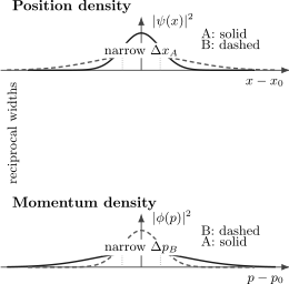
Two Gaussian states illustrate Fourier scaling. The solid state is narrower in position and broader in momentum; the dashed state has the reciprocal pattern. Translating either curve changes its mean but not its width.

The general transform machinery is developed in Fourier Transform and Wave Packets.

Scaling Makes the Reciprocal Width Exact

Let $a>0$ and define a rescaled normalized state

$$\psi_a(x) = \frac1{\sqrt a} \psi\!\left(\frac{x}{a}\right).$$

Its momentum wavefunction is

$$\phi_a(p) = \sqrt a\,\phi(ap).$$

If the original means vanish, direct substitution gives

$$\Delta_{psi_a}x = a\,\Delta_\psi x,$$

and

$$\Delta_{psi_a}p = \frac1a\,\Delta_\psi p.$$

Thus

$$\Delta_{psi_a}x\, \Delta_{psi_a}p = \Delta_\psi x\, \Delta_\psi p.$$

Narrowing the position profile by a factor $a<1$ broadens the momentum profile by exactly $1/a$. Scaling alone does not guarantee saturation; it preserves whatever uncertainty product the original shape had.

Equality Condition and the Gaussian

For nonzero variances, Robertson equality requires the centered fluctuation vectors to be proportional with a purely imaginary coefficient. Write

$$(x-x_0)\psi = -i\lambda (p-p_0)\psi, \qquad \lambda>0.$$

Using $p=-i\hbar d/dx$ gives the first-order equation

$$\frac{d\psi}{dx} = \left[ -\frac{x-x_0}{\lambda\hbar} + \frac{ip_0}{\hbar} \right] \psi.$$

Its normalizable solutions are Gaussians. Writing

$$\lambda = \frac{2\sigma_x^2}{\hbar},$$

one obtains

$$\begin{aligned} \psi(x) &= \frac{e^{i\chi}} {(2\pi\sigma_x^2)^{1/4}} \\ &\quad\times \exp\!\left[ -\frac{(x-x_0)^2}{4\sigma_x^2} \right] \\ &\quad\times \exp\!\left[ \frac{ip_0(x-x_0)}{\hbar} \right], \end{aligned}$$

where $\chi$ is an irrelevant global phase.

The probability density is

$$|\psi(x)|^2 = \frac1{\sqrt{2\pi\sigma_x^2}} \exp\!\left[ -\frac{(x-x_0)^2}{2\sigma_x^2} \right],$$

so

$$\Delta x=\sigma_x.$$

Fourier transformation gives a Gaussian centered at $p_0$ with

$$\Delta p = \frac\hbar{2\sigma_x}.$$

Hence

$$\Delta x\,\Delta p = \frac\hbar2.$$

Translations $x_0$, boosts $p_0$, and a global phase do not affect the uncertainty product. Up to those changes and the width parameter, the uncorrelated Gaussian is the normalized equality state on the line.

The packet’s free evolution and its relation to coherent states belong to Minimum-Uncertainty Wave Packets and Gaussian Wave Packets.

Correlated Gaussians and the Stronger Relation

Consider the chirped Gaussian

$$\begin{aligned} \psi_\eta(x) &= \frac1{(2\pi\sigma_x^2)^{1/4}} \\ &\quad\times \exp\!\left[ \begin{aligned} &-\frac{1-i\eta}{4\sigma_x^2}(x-x_0)^2 \\ &+\frac{ip_0(x-x_0)}{\hbar} \end{aligned} \right], \end{aligned}$$

where $\eta\in\mathbb R$. Its position density is unchanged, but the quadratic phase correlates position and momentum. Direct differentiation gives

$$(p-p_0)\psi_\eta = \frac{\hbar(\eta+i)}{2\sigma_x^2} (x-x_0)\psi_\eta.$$

Therefore

$$(\Delta x)^2=\sigma_x^2,$$ $$(\Delta p)^2 = \frac{\hbar^2}{4\sigma_x^2} (1+\eta^2),$$

and

$$C(x,p)=\frac{\eta\hbar}{2}.$$

These quantities satisfy

$$(\Delta x)^2(\Delta p)^2 - C(x,p)^2 = \frac{\hbar^2}{4}.$$

Thus every $\psi_\eta$ saturates Robertson–Schrödinger, while only $\eta=0$ saturates the simpler product relation. A state can be a minimum uncertainty state for the determinant bound without minimizing $\Delta x\,\Delta p$ itself.

Physical Meaning of Narrowing a Packet

A small $\Delta x$ means that repeated ideal position measurements on identically prepared systems have a distribution concentrated near $x_0$ in the root-mean-square sense. It does not mean that the wavefunction has compact support or that every outcome lies in an interval of width $2\Delta x$.

The inequality gives

$$\Delta p \ge \frac\hbar{2\Delta x}.$$

This concerns spread about $p_0$, not the size of $p_0$. A packet can have a large mean momentum and a small momentum spread, or zero mean momentum and a large spread.

For a free particle of mass $m$,

$$\langle T\rangle = \frac{\langle p^2\rangle}{2m} = \frac{p_0^2+(\Delta p)^2}{2m}.$$

Consequently,

$$\langle T\rangle \ge \frac{p_0^2}{2m} + \frac{\hbar^2}{8m(\Delta x)^2}.$$

Localization therefore carries a kinetic-energy cost. For an electron with $p_0=0$ and $\Delta x=1\,\text{Å}$, the lower-bound contribution is about $0.95\,\mathrm{eV}$.

Idealized Sharp States Are Not Counterexamples

Momentum plane waves

An ideal plane wave

$$\psi_p(x) \propto e^{ipx/\hbar}$$

has a sharp generalized momentum but is not square integrable on $\mathbb R$. It has no finite position variance. Normalized packets can approach a sharp momentum distribution only by spreading farther in position.

Position eigenkets

An ideal position eigenket has wavefunction proportional to

$$\delta(x-x_0).$$

It is a distribution rather than a vector in $L^2(\mathbb R)$. Its Fourier amplitude has constant magnitude, so it does not define a normalizable finite-variance momentum distribution.

Infinite-variance states

Some normalized states have heavy tails and infinite $\Delta x$ or $\Delta p$. The variance product is then not a useful finite diagnostic. This does not violate the theorem; it lies outside the finite-moment setting in which the numerical product is defined.

Higher Dimensions and Directional Pairs

For Cartesian components,

$$[x_i,p_j] = i\hbar\delta_{ij}I.$$

Therefore

$$\Delta x_i\,\Delta p_i \ge \frac\hbar2$$

for each matched component. Distinct components commute:

$$[x_i,p_j]=0 \qquad(i\ne j),$$

so this commutator supplies no positive lower bound for their product.

For real vectors $\mathbf u$ and $\mathbf v$, define

$$X_{\mathbf u} = \mathbf u\cdot\mathbf x, \qquad P_{\mathbf v} = \mathbf v\cdot\mathbf p.$$

Then

$$[X_{\mathbf u},P_{\mathbf v}] = i\hbar (\mathbf u\cdot\mathbf v)I,$$

and

$$\Delta X_{\mathbf u}\, \Delta P_{\mathbf v} \ge \frac\hbar2 |\mathbf u\cdot\mathbf v|.$$

The bound depends only on the overlap of the two directions.

Preparation Uncertainty Is Not Error–Disturbance

The theorem can be tested by preparing many copies of $\rho$. Position can be measured on one subensemble and momentum on another. Their empirical widths, after correcting for known detector effects, estimate $\Delta x$ and $\Delta p$.

No first measurement is required to disturb a second measurement in this protocol. A sequential error–disturbance experiment asks different questions about an apparatus, its resolution, and its state-update map.

Heisenberg’s microscope was historically important for motivating operational limits, but the Kennard–Robertson variance inequality is a theorem about prepared-state distributions. The historical development belongs to Uncertainty: Historical Origin.

Domain and Boundary Conditions

Position and momentum are unbounded. A sufficient whole-line setting for the vector proof requires

$$x\psi\in L^2(\mathbb R),$$ $$\psi'\in L^2(\mathbb R),$$

and a representative for which the integration-by-parts boundary term

$$\left[ (x-x_0)|\psi(x)|^2 \right]_{-\infty}^{\infty}$$

vanishes. Schwartz wavefunctions satisfy these conditions comfortably.

The direct vector proof needs $\psi$ in the common form domain of $x$ and $p$. Writing

$$\langle\psi|[x,p]|\psi\rangle$$

as an ordinary operator expectation can require stronger product-domain conditions. The weak overlap proof avoids assuming that both $xp\psi$ and $px\psi$ exist as Hilbert-space vectors.

Boundary conditions can alter the story:

• on a finite interval, self-adjoint momentum realizations depend on boundary conditions, and multiplication by $x$ may not preserve their domains;
• on a circle, a globally defined angle observable is not an ordinary Cartesian position operator;
• on a lattice or finite cyclic space, position and quasimomentum have discrete or periodic spectra and obey modified uncertainty relations;
• with gauge fields, canonical momentum and kinetic momentum are different observables.

The formula $\Delta x\,\Delta p\ge\hbar/2$ should therefore be attached to the canonical pair on the line, not exported unchanged to every coordinate called “position.”

Practical Checks

When using the relation:

1. Confirm that $x$ and $p$ are the canonical operators for the stated configuration space.
2. Normalize the state and verify that both second moments are finite.
3. Keep the means $x_0$ and $p_0$ separate from the spreads.
4. Use one Fourier convention consistently.
5. Check the dimensions: $\Delta x\,\Delta p$ has units of action.
6. Inspect boundary terms or use the domain-safe weak form.
7. Include covariance when discussing equality or chirped states.
8. Do not infer detector error or sequential disturbance without a measurement model.
9. Test limiting cases such as broad packets, narrow packets, and Gaussian saturation.

Common Misstatements

• “The particle has exact $x$ and $p$, but observation hides them.” The variance theorem itself concerns state-assigned outcome distributions and makes no such hidden-value assertion.
• “Uncertainty is caused only by the observer disturbing the particle.” The preparation inequality exists before a measurement sequence is chosen.
• “$\Delta x$ is the resolution of the position detector.” It is the ideal Born-distribution standard deviation.
• “Small $\Delta x$ means large $\langle p\rangle$.” It requires a large momentum spread, not a large mean.
• “All Gaussians satisfy $\Delta x\,\Delta p=\hbar/2$.” Quadratic-phase Gaussians generally have a larger product while saturating the covariance determinant bound.
• “Every state saturates the relation.” Most wavefunctions lie strictly above the bound.
• “A plane wave violates the theorem because $\Delta p=0$.” It is not a normalized finite-$\Delta x$ state on the line.
• “The theorem says the particle is somewhere inside $x_0\pm\Delta x$.” A standard deviation is not a compact support interval.
• “The same formula applies unchanged to angle and angular momentum.” Periodic coordinates require separate domain-aware relations.
• “Energy–time uncertainty follows by replacing $x$ with $t$.” Time is not a universal position-like operator in ordinary quantum mechanics.

Canonical Boundaries

This page owns the canonical variance theorem, its Fourier and wavefunction derivations, Gaussian equality condition, covariance refinement, and line-domain caveats. Nearby pages own specialized developments:

• General Uncertainty Relations owns the abstract Cauchy–Schwarz proof and multi-observable matrix form.
• Canonical Commutation Relations owns translations, Weyl relations, and representation theory.
• Momentum-Space Representation owns the momentum wavefunction and transform conventions in Core Formalism.
• Gaussian Wave Packets owns free evolution and spreading.
• Minimum-Uncertainty Wave Packets owns dynamical uses, chirp evolution, and coherent-state connections.
• Energy–Time Uncertainty owns timescale and lifetime–linewidth relations.

Summary

• Every normalized whole-line state with finite canonical variances obeys $\Delta x\,\Delta p\ge\hbar/2$.
• The bound is state independent because $[x,p]=i\hbar I$.
• The theorem is simultaneously an operator inequality and a Fourier width theorem.
• Translation and boost change the means but not the variances.
• Rescaling position by $a$ rescales momentum width by $1/a$.
• Uncorrelated Gaussians are the normalized equality states for the product relation on the line.
• Chirped Gaussians saturate Robertson–Schrödinger but generally not the simpler product bound.
• Plane waves and position eigenkets are distributional idealizations, not finite-variance counterexamples.
• Preparation spread, detector error, and measurement disturbance are distinct notions.
• Unbounded operators, boundaries, periodic coordinates, and gauge fields require explicit domain and observable choices.

References

• W. Heisenberg, “Über den anschaulichen Inhalt der quantentheoretischen Kinematik und Mechanik,” Zeitschrift für Physik 43, 172–198, 1927, doi:10.1007/BF01397280.
• E. H. Kennard, “Zur Quantenmechanik einfacher Bewegungstypen,” Zeitschrift für Physik 44, 326–352, 1927, doi:10.1007/BF01391200.
• H. P. Robertson, “The Uncertainty Principle,” Physical Review 34, 163–164, 1929, doi:10.1103/PhysRev.34.163.
• E. Schrödinger, “Zum Heisenbergschen Unschärfeprinzip,” Sitzungsberichte der Preußischen Akademie der Wissenschaften, Physikalisch-mathematische Klasse, 296–303, 1930.
• G. B. Folland and A. Sitaram, “The Uncertainty Principle: A Mathematical Survey,” Journal of Fourier Analysis and Applications 3, 207–238, 1997.
• L. E. Ballentine, Quantum Mechanics: A Modern Development, 2nd ed., World Scientific, 2014.
• R. Shankar, Principles of Quantum Mechanics, 2nd ed., Springer, 1994.
• B. C. Hall, Quantum Theory for Mathematicians, Springer, 2013.
• M. Reed and B. Simon, Methods of Modern Mathematical Physics, Vol. I: Functional Analysis, rev. ed., Academic Press, 1980.
• P. Busch, P. Lahti, J.-P. Pellonpää, and K. Ylinen, Quantum Measurement, Springer, 2016.

Exercises

Exercise 1: State-independent Robertson bound

Starting from Robertson and $[x,p]=i\hbar I$, derive the position–momentum uncertainty relation. Identify exactly where normalization is used.

Solution

Robertson gives

$$\Delta_\psi x\,\Delta_\psi p \ge \frac12 \left\lvert \langle[x,p]\rangle_\psi \right\rvert.$$

The canonical relation implies

$$\langle[x,p]\rangle_\psi = i\hbar\langle I\rangle_\psi.$$

Normalization is used in

$$\langle I\rangle_\psi = \langle\psi|\psi\rangle =1.$$

Hence

$$\Delta_\psi x\,\Delta_\psi p \ge \frac12|i\hbar| = \frac\hbar2.$$

Exercise 2: The integration-by-parts constant

Assume $\psi$ is normalized, differentiable, and decays sufficiently rapidly. Show that

$$\operatorname{Re} \int_{-\infty}^{\infty} (x-x_0)\psi^*(x)\psi'(x)\,dx = -\frac12.$$

Explain how this fixes the constant $\hbar/2$.

Solution

Let the integral be $I$. Then

$$\begin{aligned} 2\operatorname{Re}I &= I+I^*\\ &= \int_{-\infty}^{\infty} (x-x_0) \frac{d}{dx}|\psi(x)|^2\,dx. \end{aligned}$$

Integration by parts gives

$$\begin{aligned} 2\operatorname{Re}I &= \left[ (x-x_0)|\psi(x)|^2 \right]_{-\infty}^{\infty} \\ &\quad- \int_{-\infty}^{\infty}|\psi(x)|^2\,dx \\ &=-1. \end{aligned}$$

Thus $\operatorname{Re}I=-1/2$. The centered position–momentum overlap is $-i\hbar I$, whose imaginary part is $\hbar/2$. Cauchy–Schwarz must therefore bound its modulus by at least $\hbar/2$.

Exercise 3: Gaussian saturation

For

$$\begin{aligned} \psi(x) &= \frac1{(2\pi\sigma^2)^{1/4}} \exp\!\left[ -\frac{(x-x_0)^2}{4\sigma^2} \right] \\ &\quad\times \exp\!\left[ \frac{ip_0(x-x_0)}{\hbar} \right], \end{aligned}$$

compute $\Delta x$ and $\Delta p$ without performing the full Fourier transform.

Solution

The density is a normal distribution of variance $\sigma^2$, so

$$\Delta x=\sigma.$$

Differentiate the wavefunction:

$$\psi' = \left[ -\frac{x-x_0}{2\sigma^2} + \frac{ip_0}{\hbar} \right]\psi.$$

Therefore

$$(p-p_0)\psi = \frac{i\hbar(x-x_0)}{2\sigma^2}\psi.$$

Taking the norm gives

$$\begin{aligned} (\Delta p)^2 &= \frac{\hbar^2}{4\sigma^4} \langle(x-x_0)^2\rangle \\ &= \frac{\hbar^2}{4\sigma^2}. \end{aligned}$$

Thus $\Delta p=\hbar/(2\sigma)$ and the product is $\hbar/2$.

Exercise 4: Fourier scaling

For $a>0$, let

$$\psi_a(x) = a^{-1/2}\psi(x/a).$$

Derive $\phi_a(p)=a^{1/2}\phi(ap)$ and show how the two variances scale.

Solution

Substitute $x=ay$ into the Fourier transform:

$$\begin{aligned} \phi_a(p) &= \frac1{\sqrt{2\pi\hbar}} \\ &\quad\times \int e^{-ipx/\hbar} a^{-1/2}\psi(x/a)\,dx \\ &= a^{1/2} \frac1{\sqrt{2\pi\hbar}} \\ &\quad\times \int e^{-i(ap)y/\hbar}\psi(y)\,dy \\ &= a^{1/2}\phi(ap). \end{aligned}$$

Changing variables in the second moments gives

$$\Delta_{psi_a}x=a\Delta_\psi x,$$

and

$$\Delta_{psi_a}p=\frac1a\Delta_\psi p.$$

Their product is unchanged.

Exercise 5: A chirped Gaussian

For the state $\psi_\eta$ defined in the text, verify

$$(p-p_0)\psi_\eta = \frac{\hbar(\eta+i)}{2\sigma_x^2} (x-x_0)\psi_\eta,$$

then compute $\Delta p$ and $C(x,p)$.

Solution

Differentiation gives

$$\psi_\eta' = \left[ -\frac{1-i\eta}{2\sigma_x^2}(x-x_0) + \frac{ip_0}{\hbar} \right] \psi_\eta.$$

Applying $-i\hbar d/dx-p_0$ yields the stated relation. Its squared norm is

$$\begin{aligned} (\Delta p)^2 &= \frac{\hbar^2|\eta+i|^2}{4\sigma_x^4} \langle(x-x_0)^2\rangle \\ &= \frac{\hbar^2(1+\eta^2)}{4\sigma_x^2}. \end{aligned}$$

The centered overlap is

$$\begin{aligned} \langle(x-x_0)(p-p_0)\rangle &= \frac{\hbar(\eta+i)}{2\sigma_x^2} \\ &\quad\times \langle(x-x_0)^2\rangle \\ &= \frac\hbar2(\eta+i). \end{aligned}$$

Its real part is the symmetrized covariance:

$$C(x,p)=\frac{\eta\hbar}{2}.$$

Substitution verifies saturation of the determinant relation.

Exercise 6: Localization energy scale

For a free particle with $p_0=0$, show that

$$\langle T\rangle \ge \frac{\hbar^2}{8m(\Delta x)^2}.$$

Estimate the bound for an electron localized to $\Delta x=1\,\text{Å}$.

Solution

Since $p_0=0$,

$$\langle T\rangle = \frac{(\Delta p)^2}{2m}.$$

The uncertainty relation gives

$$(\Delta p)^2 \ge \frac{\hbar^2}{4(\Delta x)^2},$$

so

$$\langle T\rangle \ge \frac{\hbar^2}{8m(\Delta x)^2}.$$

Using $m_e\simeq9.11\times10^{-31}\,\mathrm{kg}$ and $\Delta x=10^{-10}\,\mathrm m$ gives

$$\langle T\rangle \gtrsim 1.53\times10^{-19}\,\mathrm J \simeq0.95\,\mathrm{eV}.$$

Exercise 7: Directional uncertainty in three dimensions

Let $\mathbf u$ and $\mathbf v$ be unit vectors. Derive

$$\Delta(\mathbf u\cdot\mathbf x)\, \Delta(\mathbf v\cdot\mathbf p) \ge \frac\hbar2|\mathbf u\cdot\mathbf v|.$$

What does Robertson give when the directions are orthogonal?

Solution

Using $[x_i,p_j]=i\hbar\delta_{ij}I$,

$$\begin{aligned} [\mathbf u\cdot\mathbf x, \mathbf v\cdot\mathbf p] &= \sum_{i,j}u_iv_j[x_i,p_j] \\ &= i\hbar \sum_i u_iv_i I \\ &= i\hbar(\mathbf u\cdot\mathbf v)I. \end{aligned}$$

Robertson gives the stated bound. If the directions are orthogonal, the commutator vanishes and this particular relation gives only the trivial lower bound zero. It does not require either variance to vanish.

Exercise 8: Why the boundary term matters

Repeat the integration-by-parts step on an interval $[0,L]$. Show that

$$\begin{aligned} 2\operatorname{Re}I &= \left[ (x-x_0)|\psi(x)|^2 \right]_{0}^{L} -1. \end{aligned}$$

Explain why the whole-line proof cannot simply be copied to arbitrary boundary conditions.

Solution

The calculation is identical except that the endpoints are finite:

$$\begin{aligned} I+I^* &= \int_0^L (x-x_0) \frac{d}{dx}|\psi(x)|^2\,dx \\ &= \left[ (x-x_0)|\psi(x)|^2 \right]_0^L \\ &\quad- \int_0^L|\psi(x)|^2\,dx. \end{aligned}$$

Normalization makes the last integral one, yielding the stated result. The endpoint contribution need not vanish for periodic or other self-adjoint boundary conditions. In addition, multiplication by $x$ may not preserve the domain of the chosen momentum operator. The observable domains and boundary conditions must therefore be analyzed before asserting the whole-line constant.