Noncommuting Observables

Two observables are noncommuting when their operators satisfy

$$[A,B] = AB-BA \ne0.$$

This is an operator statement: somewhere in the Hilbert space, the two orderings act differently. For finite-dimensional sharp observables, it has several equivalent physical consequences:

• the observables have no complete orthonormal basis of simultaneous eigenvectors;
• their spectral projectors admit no single sharp joint measurement;
• an ideal measurement of one can change the statistics of a later measurement of the other;
• ordered products and ordered measurement probabilities cannot generally be replaced by one classical joint distribution.

These statements are related, but they are not interchangeable. Noncommutativity is state independent, while uncertainty bounds and observed order effects can depend on the state. Preparation uncertainty describes two distributions assigned to one input state, while measurement disturbance describes a physical intervention. Generalized, unsharp measurements can also be jointly measurable even when some of their effects do not commute.

The reliable conclusion is therefore not that “both quantities are unknowable.” It is that the two sharp observables do not belong to one common classical measurement context.

Scope and Conventions

Most of this page assumes a finite-dimensional complex Hilbert space and two self-adjoint operators with spectral decompositions

$$A = \sum_a aP_a, \qquad B = \sum_b bQ_b.$$

The projectors $P_a$ and $Q_b$ refer to complete eigenspaces, including all degeneracy. They obey

$$P_aP_{a'} = \delta_{aa'}P_a, \qquad \sum_aP_a=I,$$

and analogous relations for the $Q_b$.

Three levels of description will be kept separate:

1. Algebra: whether $[A,B]$ vanishes as an operator.
2. Sharp measurement structure: whether all $P_a$ commute with all $Q_b$.
3. A particular experiment: whether a chosen state and two chosen measurement implementations exhibit different statistics when reordered.

For self-adjoint matrices, the first two criteria are equivalent. The third is more specific: noncommutation guarantees that an order-sensitive experiment can be found, not that every input state and every reported statistic must show an order effect.

The algebra of the bracket itself belongs to Commutators. The full ordered-probability calculation belongs to Sequential Measurements. This page concentrates on what noncommutation means physically.

Order of Operator Actions

Operator products act from right to left:

$$AB|\psi\rangle = A\left(B|\psi\rangle\right),$$

whereas

$$BA|\psi\rangle = B\left(A|\psi\rangle\right).$$

If $[A,B]\ne0$, there is at least one vector in the common domain for which these outputs differ. Equivalently, there is some $|\psi\rangle$ such that

$$AB|\psi\rangle \ne BA|\psi\rangle.$$

That statement concerns operator composition. It must not be read too literally as a measurement recipe. In particular, the product $AB$ is not by itself the state-update map for “measure $B$, then measure $A$.” Sequential measurements require outcome projectors or, more generally, quantum instruments.

There is another useful warning. If $A$ and $B$ are Hermitian, then

$$(AB)^{\dagger}=BA.$$

Consequently,

$$AB=(AB)^{\dagger} \quad\Longleftrightarrow\quad [A,B]=0.$$

For noncommuting observables, the ordered product $AB$ is generally not itself an observable. Its Hermitian and anti-Hermitian parts are

$$\frac12(AB+BA) = \frac12\{A,B\},$$

and

$$\frac12(AB-BA) = \frac12[A,B].$$

The first is the symmetrized product used in covariance; the second records order sensitivity. See Anticommutators for the symmetric part.

Sharp Incompatibility

For finite-dimensional self-adjoint operators, the following statements are equivalent:

1. $[A,B]=0$.
2. $[P_a,Q_b]=0$ for every $a,b$.
3. There is a complete orthonormal basis of simultaneous eigenvectors.
4. The two projective measurements have a common projective refinement.

Therefore

$$[A,B]\ne0$$

means that at least one pair of spectral projectors fails to commute and that no single projective measurement can reproduce both sharp observables as marginals.

The projector formulation is the operationally precise one. Eigenvalue degeneracy does not create a loophole: each $P_a$ projects onto the whole $a$-eigenspace. What degeneracy can do is allow the two observables to share some eigenvectors or invariant subspaces without sharing a complete basis.

The commuting theorem and its proof are developed in Compatible Observables.

No Complete Shared Eigenbasis

Suppose an orthonormal basis $\{|n\rangle\}$ diagonalized both observables:

$$A|n\rangle=a_n|n\rangle, \qquad B|n\rangle=b_n|n\rangle.$$

Then every basis vector would satisfy

$$AB|n\rangle = a_nb_n|n\rangle = BA|n\rangle.$$

By linearity, $AB=BA$ on the whole space. The contrapositive gives the useful test:

$$\begin{gathered} [A,B]\ne0 \\ \Longrightarrow \\ \text{no complete simultaneous eigenbasis}. \end{gathered}$$

The word complete is essential. If one normalized state happens to satisfy

$$A|\psi\rangle=a|\psi\rangle, \qquad B|\psi\rangle=b|\psi\rangle,$$

then

$$[A,B]|\psi\rangle=0.$$

This does not force the commutator to vanish on vectors orthogonal to $|\psi\rangle$.

A three-dimensional example

In the basis $\{|1\rangle,|2\rangle,|3\rangle\}$, let

$$A = \begin{pmatrix} 0&0&0\\ 0&1&0\\ 0&0&2 \end{pmatrix},$$

and

$$B = \begin{pmatrix} 3&0&0\\ 0&0&1\\ 0&1&0 \end{pmatrix}.$$

Both matrices are Hermitian, and $|1\rangle$ is a common eigenvector:

$$A|1\rangle=0, \qquad B|1\rangle=3|1\rangle.$$

Nevertheless,

$$[A,B] = \begin{pmatrix} 0&0&0\\ 0&0&-1\\ 0&1&0 \end{pmatrix} \ne0.$$

The observables agree on one one-dimensional sector but differ in how they act on the span of $|2\rangle$ and $|3\rangle$. A single common eigenvector is therefore a state-specific fact, not compatibility of the observables.

The finer distinction between common eigenvectors, common eigenspaces, and a complete common basis is the subject of Simultaneous Eigenstates.

Three State-Dependent Tests

The following statements have decreasing strength:

$$[A,B]=0,$$ $$[A,B]|\psi\rangle=0,$$

and

$$\langle\psi|[A,B]|\psi\rangle=0.$$

The first is an operator identity. The second says that the two orderings agree on one state. The third says only that their difference has zero expectation in that state.

Neither state-dependent equality proves compatibility. For example,

$$[\sigma_x,\sigma_y]=2i\sigma_z\ne0,$$

but in $|+x\rangle$,

$$\langle+x|[\sigma_x,\sigma_y]|+x\rangle = 2i\langle+x|\sigma_z|+x\rangle =0.$$

This hierarchy explains why the expectation of a commutator is not a scalar measure of how incompatible two observables are.

Sequential Projective Measurements

Let the initial state be a density operator $\rho$. An ideal projective measurement of $A$ first, followed by one of $B$, has ordered joint probability

$$\begin{aligned} p_{A\to B}(a,b) &= \operatorname{Tr} \left( Q_bP_a\rho P_a \right)\\ &= \operatorname{Tr} \left( \rho P_aQ_bP_a \right). \end{aligned}$$

Reversing the apparatus order gives

$$\begin{aligned} p_{B\to A}(b,a) &= \operatorname{Tr} \left( P_aQ_b\rho Q_b \right)\\ &= \operatorname{Tr} \left( \rho Q_bP_aQ_b \right). \end{aligned}$$

These are probabilities for two different experiments. If the projectors commute, then

$$P_aQ_bP_a = P_aQ_b = Q_bP_aQ_b,$$

so both orders reduce to the joint probability

$$p(a,b) = \operatorname{Tr}(\rho P_aQ_b).$$

If some $P_a$ and $Q_b$ do not commute, the two ordered expressions need not agree. The first measurement changes which state enters the second Born-rule calculation.

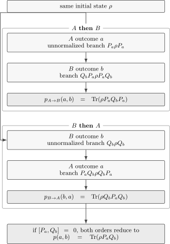
The sequences $A\to B$ and $B\to A$ contain different projector products. When every $P_a$ commutes with every $Q_b$, both branches reduce to the common sharp joint effect $P_aQ_b$.

Possibility is not universality

Noncommutation does not imply

$$p_{A\to B}(a,b) \ne p_{B\to A}(b,a)$$

for every $\rho,a,b$. Symmetry, a special input state, or a particular outcome can make the two numbers equal. The correct global statement is that noncommuting sharp observables do not admit order-independent joint projective statistics for all states.

This distinction is experimentally important. A null order effect in one preparation is not evidence that the observables commute; one must vary the preparation or test the operator/projector relation directly.

Unread Measurements and Disturbance

Suppose the $A$ outcome is not retained. The ideal nonselective Lüders channel is

$$\mathcal L_A(\rho) = \sum_aP_a\rho P_a.$$

The probability of a later $B$ outcome becomes

$$\begin{aligned} p_A(b) &= \operatorname{Tr} \left[ Q_b\mathcal L_A(\rho) \right]\\ &= \operatorname{Tr} \left[ \rho\mathcal L_A^{*}(Q_b) \right], \end{aligned}$$

where the dual map acts as

$$\mathcal L_A^{*}(Q_b) = \sum_aP_aQ_bP_a.$$

The unread $A$ measurement leaves the $B$ statistics unchanged for every state exactly when

$$\mathcal L_A^{*}(Q_b)=Q_b$$

for every $b$. For projective $A$ and $B$, this is equivalent to

$$[P_a,Q_b]=0$$

for all $a,b$. Thus noncommuting sharp observables permit a preparation for which an unread ideal measurement of one changes a later distribution of the other.

The channel formula also shows why “the result was ignored” does not mean “no measurement occurred.” Discarding the classical record sums the conditioned branches; it does not undo the physical interaction.

For realistic apparatuses, a POVM specifies outcome probabilities but not the postmeasurement state. The full instrument is needed to predict later statistics. That more general distinction belongs to Compatible, Incompatible, and Sequential Measurements.

Spin One-Half Example

For a spin-$1/2$ particle,

$$S_i=\frac{\hbar}{2}\sigma_i.$$

The Pauli algebra gives

$$[S_x,S_z] = -i\hbar S_y,$$

so $S_x$ and $S_z$ are noncommuting sharp observables.

Prepare $|+z\rangle$. A direct $S_z$ measurement is certain to return $+\hbar/2$. If an unread $S_x$ measurement is inserted first, the state becomes

$$\begin{aligned} \mathcal L_x(|+z\rangle\langle+z|) &= P_{+x}|+z\rangle\langle+z|P_{+x}\\ &\quad+ P_{-x}|+z\rangle\langle+z|P_{-x}\\ &= \frac12I. \end{aligned}$$

The later $S_z$ probabilities are therefore

$$p(+z)=\frac12, \qquad p(-z)=\frac12.$$

The comparison is operational:

$$\begin{array}{c|c} \text{sequence} & \text{final }S_z\text{ distribution}\\ \hline S_z & (1,0)\\ S_x\text{ unread},\ S_z & (1/2,1/2) \end{array}$$

Changing representation would not have this effect. A basis change rewrites the same state and operators; inserting an $S_x$ apparatus performs a new physical operation.

General two-axis formula

Let

$$P_s^{(\mathbf n)} = \frac12 \left( I+s\,\mathbf n\cdot\boldsymbol\sigma \right),$$

where $s\in\{+1,-1\}$, and let the input state have Bloch vector $\mathbf r$:

$$\rho = \frac12 \left( I+\mathbf r\cdot\boldsymbol\sigma \right).$$

Measuring along $\mathbf n$ and then $\mathbf m$ gives

$$\begin{aligned} p_{\mathbf n\to\mathbf m}(s,t) &= \frac14 \left(1+s\,\mathbf r\cdot\mathbf n\right) \\ &\quad\times \left(1+st\,\mathbf n\cdot\mathbf m\right). \end{aligned}$$

The reversed order gives

$$\begin{aligned} p_{\mathbf m\to\mathbf n}(t,s) &= \frac14 \left(1+t\,\mathbf r\cdot\mathbf m\right) \\ &\quad\times \left(1+st\,\mathbf n\cdot\mathbf m\right). \end{aligned}$$

The conditional factor is symmetric, but the first-outcome factor probes a different component of the input Bloch vector. This makes both the potential order dependence and its state dependence explicit.

The matrix identities used here are collected in Pauli Matrices.

Why There Is No Sharp Joint Probability

For commuting projectors, the joint alternatives are

$$G_{ab}=P_aQ_b.$$

They are projectors, sum to the identity, and have the correct marginals:

$$\sum_bG_{ab}=P_a, \qquad \sum_aG_{ab}=Q_b.$$

Conversely, suppose a projective measurement $\{G_{ab}\}$ had these marginals. Orthogonality of its outcomes would give

$$P_aQ_b = G_{ab} = Q_bP_a.$$

Thus a common sharp joint measurement would force all spectral projectors to commute. Noncommuting sharp observables therefore have no state-independent joint PVM with their original distributions as marginals.

A classical coupling is not a joint quantum measurement

For one fixed state, the separate Born distributions

$$p_A(a)=\operatorname{Tr}(\rho P_a), \qquad p_B(b)=\operatorname{Tr}(\rho Q_b)$$

can always be embedded in some artificial classical joint distribution. For example, $p_A(a)p_B(b)$ has the right marginals. But that choice is not selected by the quantum experiment, does not reproduce ordered measurement statistics in general, and need not respect any physically accessible joint correlations.

The obstruction is not the elementary mathematics of coupling two lists of probabilities. It is the absence of one sharp quantum measurement whose marginals are the specified observables for every input state.

Ordered quasiprobabilities

One can define an ordered quantity

$$q(a,b) = \operatorname{Tr}(\rho Q_bP_a).$$

It has the correct marginals:

$$\begin{aligned} \sum_bq(a,b)&=p_A(a),\\ \sum_aq(a,b)&=p_B(b). \end{aligned}$$

For noncommuting projectors, however, $Q_bP_a$ need not be Hermitian, so $q(a,b)$ can be negative or complex. Such Kirkwood–Dirac-type quantities are useful ordered quasiprobabilities, not ordinary probabilities of jointly preexisting sharp values.

Generalized Measurements Are Broader

The equivalence between commutation and joint measurability applies to sharp projective observables. A generalized measurement uses positive effects $E_a$ satisfying

$$E_a\ge0, \qquad \sum_aE_a=I,$$

without requiring $E_a^2=E_a$.

Two POVMs $\{E_a\}$ and $\{F_b\}$ are jointly measurable if there is a parent POVM $\{G_{ab}\}$ such that

$$\sum_bG_{ab}=E_a, \qquad \sum_aG_{ab}=F_b.$$

The effects $E_a$ and $F_b$ need not commute. Sufficiently noisy or unsharp versions of incompatible spin components can possess such a parent POVM. What is lost is the simultaneous sharpness of the original projective alternatives.

This is not an exception to the sharp-observable theorem; it is a broader measurement model. The distinction is developed in POVMs: First Encounter and Unsharp Measurements.

Preparation Uncertainty Is Not Disturbance

For a state $\rho$, the Robertson relation says

$$\Delta_\rho A\,\Delta_\rho B \ge \frac12 \left\lvert \operatorname{Tr}(\rho[A,B]) \right\rvert.$$

This compares the standard deviations of two hypothetical outcome distributions prepared from the same input state. It does not require that $A$ be measured first, and it is not a formula for how much an $A$ apparatus disturbs $B$.

Four notions should be distinguished:

• incompatibility: a state-independent relation between observables or measurements;
• preparation uncertainty: a tradeoff between distributions in one input state;
• measurement disturbance: a change caused by a specified instrument;
• joint-measurement error: the accuracy with which one apparatus approximates two target observables.

They influence one another, but they answer different experimental questions.

A vanishing Robertson bound

The Robertson lower bound is state dependent. For $A=\sigma_x$, $B=\sigma_y$, and $\rho=|+x\rangle\langle+x|$,

$$\Delta_\rho\sigma_x=0, \qquad \Delta_\rho\sigma_y=1,$$

while

$$\operatorname{Tr} \left( \rho[\sigma_x,\sigma_y] \right) =0.$$

The inequality becomes $0\ge0$, even though $[\sigma_x,\sigma_y]\ne0$. The state is sharp in one observable, not both. The bound is simply noninformative about their global incompatibility.

By contrast, the canonical relation

$$[x,p]=i\hbar I$$

has the same nonzero expectation in every normalized state in the relevant domains, producing

$$\Delta x\,\Delta p \ge \frac{\hbar}{2}.$$

The derivation, covariance term, and equality conditions belong to General Uncertainty Relations. The domain-sensitive canonical case belongs to Position–Momentum Uncertainty.

Disturbance depends on the instrument

A sharp Lüders measurement supplies one standard state-update rule, but an observable does not uniquely specify every apparatus that measures it. Two instruments can have the same outcome probabilities and different postmeasurement states. An apparatus can also add avoidable disturbance after recording its result.

Accordingly, the Robertson relation should never be advertised as a universal error–disturbance formula. Quantitative measurement-error and disturbance relations require operational definitions of error, a measurement model, and careful assumptions.

What Noncommutativity Does Not Imply

Neither observable must be indefinite in every state

An eigenstate of $A$ has $\Delta A=0$ even when $[A,B]\ne0$. What generally fails is a complete set of states that are sharp in both observables.

Every outcome need not be uniformly random

Measuring $B$ in an $A$ eigenstate produces probabilities

$$p(b|a)=\langle a|Q_b|a\rangle.$$

These probabilities depend on basis overlaps. They are uniform only for special pairs, such as mutually unbiased bases in finite dimensions.

A zero commutator expectation does not prove compatibility

The condition

$$\langle[A,B]\rangle_\rho=0$$

constrains one scalar in one state. Compatibility requires the operator, or equivalently every relevant spectral-projector commutator, to vanish.

A basis change is not a measurement

Changing coordinates transforms states and operators together and leaves all physical probabilities invariant. Inserting an apparatus applies an instrument and can change later statistics.

Noncommutation is not the same as contextuality

Noncommutation is necessary structure behind many contextuality scenarios, but a single noncommuting pair is not by itself a Kochen–Specker proof or a Bell experiment. Those claims require additional observables, compatibility contexts, and statistical constraints.

Noncommutation does not imply statistical independence fails in one fixed way

Without a sharp joint measurement there is no canonical ordinary joint law to which classical independence can be applied. Ordered, symmetrized, and quasiprobability correlations answer different questions.

Infinite-Dimensional Caveats

For bounded self-adjoint operators, $[A,B]=0$ is equivalent to commutation of their spectral measures. For unbounded observables, the products $AB$ and $BA$ may be defined only on different domains. The formal commutator has domain

$$\mathcal D([A,B]) = \mathcal D(AB) \cap \mathcal D(BA).$$

Even if $[A,B]\psi=0$ on a convenient dense test domain, it does not automatically follow that all spectral projectors commute. The robust compatibility notion is strong commutation:

$$E_A(X)E_B(Y) = E_B(Y)E_A(X)$$

for all Borel sets $X$ and $Y$.

Conversely, a nonzero commutator computed on a valid common invariant domain is strong evidence of incompatibility, but domain declarations remain part of the statement. Position and momentum require particular care because their canonical commutator cannot be realized by finite matrices and is most safely related to exponentiated Weyl operators. See Canonical Commutation Relations.

Practical Diagnostic

When a problem says that two quantities are “incompatible,” ask which claim is actually needed.

1. To compare algebraic orderings, compute $[A,B]$ on the declared domain.
2. To test joint sharp measurability, compare all spectral projectors.
3. To find common sharp states, solve the simultaneous eigenvalue equations; do not infer the answer from one expectation value.
4. To predict a sequence, use projectors or instruments in the physical order.
5. To study an unread intermediate measurement, apply the nonselective channel rather than deleting the measurement from the calculation.
6. To compare preparation spreads, use the appropriate uncertainty relation.
7. To discuss approximate joint measurements, formulate the problem with POVMs and an explicit error criterion.

This checklist prevents the word “incompatible” from carrying more meaning than the mathematics supports.

Common Mistakes

• Reading $AB$ as the complete state-update rule for two measurements.
• Assuming that noncommutation forces different ordered probabilities for every state and outcome.
• Concluding from one common eigenvector that two observables are compatible.
• Concluding from $\langle[A,B]\rangle=0$ that $[A,B]=0$.
• Saying that neither observable can ever be sharp.
• Treating the Robertson relation as a universal measurement-error or disturbance law.
• Removing an unread measurement from a sequence instead of summing its outcome branches.
• Treating a change of basis as a physical intervention.
• Interpreting $\langle AB\rangle$ as an ordinary joint moment when $AB$ is not Hermitian.
• Extending the sharp commutation criterion unchanged to general POVMs.
• Ignoring degeneracy and the difference between one common eigenvector and a complete common basis.
• Manipulating unbounded commutators without checking domains or strong spectral commutation.

Canonical Boundaries

This page owns the physical consequences and interpretive distinctions associated with noncommuting observables. Nearby pages own the detailed machinery:

• Commutators owns bracket identities, generators, and algebraic calculations.
• Compatible Observables owns the equivalence between commutation, common bases, and sharp joint refinements.
• Sequential Measurements owns conditional probabilities and ideal state-update calculations.
• General Uncertainty Relations owns the Robertson and Robertson–Schrödinger derivations.
• Correlations and Covariance owns symmetrized quantum covariance.
• Unsharp Measurements owns nonprojective effects, instruments, and the sharpness–disturbance distinction.

Summary

• $[A,B]\ne0$ means that the two operator orderings differ somewhere in the Hilbert space.
• Finite-dimensional noncommuting sharp observables have no complete common eigenbasis and no common sharp joint measurement.
• They may still share isolated eigenvectors or agree on special states.
• Ideal ordered measurements involve $P_aQ_bP_a$ and $Q_bP_aQ_b$, not merely the products $AB$ and $BA$.
• Noncommutation makes order effects possible, but special states or outcomes can hide them.
• An unread ideal measurement can alter a later incompatible distribution.
• Preparation uncertainty and measurement disturbance are distinct claims.
• A vanishing state-dependent commutator expectation does not establish compatibility.
• General POVMs can be jointly measurable without commuting effect by effect.
• Unbounded observables require domain control and strong spectral commutation.

References

• P. A. M. Dirac, The Principles of Quantum Mechanics, 4th ed., Oxford University Press, 1958.
• J. von Neumann, Mathematical Foundations of Quantum Mechanics, Princeton University Press, 1955.
• G. Lüders, “Über die Zustandsänderung durch den Meßprozeß,” Annalen der Physik 443, 322–328, 1950, doi:10.1002/andp.19504430510.
• A. Peres, Quantum Theory: Concepts and Methods, Kluwer, 1995.
• R. Shankar, Principles of Quantum Mechanics, 2nd ed., Springer, 1994.
• J. J. Sakurai and J. Napolitano, Modern Quantum Mechanics, 3rd ed., Cambridge University Press, 2020.
• P. Busch, “Unsharp Reality and Joint Measurements for Spin Observables,” Physical Review D 33, 2253–2261, 1986, doi:10.1103/PhysRevD.33.2253.
• T. Heinosaari, D. Reitzner, and P. Stano, “Notes on Joint Measurability of Quantum Observables,” Foundations of Physics 38, 1133–1147, 2008, doi:10.1007/s10701-008-9256-7.
• M. Ozawa, “Universally Valid Reformulation of the Heisenberg Uncertainty Principle on Noise and Disturbance in Measurement,” Physical Review A 67, 042105, 2003, doi:10.1103/PhysRevA.67.042105.
• P. Busch, P. Lahti, J.-P. Pellonpää, and K. Ylinen, Quantum Measurement, Springer, 2016.
• B. C. Hall, Quantum Theory for Mathematicians, Springer, 2013.
• M. Reed and B. Simon, Methods of Modern Mathematical Physics, Vol. I: Functional Analysis, rev. ed., Academic Press, 1980.

Exercises

Exercise 1: A common eigenvector without compatibility

For

$$A = \begin{pmatrix} 0&0&0\\ 0&1&0\\ 0&0&2 \end{pmatrix}, \qquad B = \begin{pmatrix} 3&0&0\\ 0&0&1\\ 0&1&0 \end{pmatrix},$$

verify that $|1\rangle=(1,0,0)^{\mathsf T}$ is a common eigenvector, compute $[A,B]$, and explain why the observables are nevertheless incompatible.

Solution

Direct multiplication gives

$$A|1\rangle=0, \qquad B|1\rangle=3|1\rangle.$$

Thus $|1\rangle$ is a common eigenvector. The ordered products are

$$AB = \begin{pmatrix} 0&0&0\\ 0&0&1\\ 0&2&0 \end{pmatrix},$$

and

$$BA = \begin{pmatrix} 0&0&0\\ 0&0&2\\ 0&1&0 \end{pmatrix}.$$

Therefore

$$[A,B] = \begin{pmatrix} 0&0&0\\ 0&0&-1\\ 0&1&0 \end{pmatrix} \ne0.$$

The commutator annihilates $|1\rangle$ but not the whole space. One common eigenvector is insufficient for simultaneous diagonalization.

Exercise 2: Ordered spin probabilities

A qubit has input state

$$\rho = \frac12 \left( I+\mathbf r\cdot\boldsymbol\sigma \right).$$

Using

$$P_s^{(\mathbf n)} = \frac12 \left( I+s\,\mathbf n\cdot\boldsymbol\sigma \right),$$

derive the probability for outcome $s$ along $\mathbf n$ followed by outcome $t$ along $\mathbf m$.

Solution

The first-outcome probability is

$$p(s) = \operatorname{Tr} \left( \rho P_s^{(\mathbf n)} \right) = \frac12 \left( 1+s\,\mathbf r\cdot\mathbf n \right).$$

After that rank-one outcome, the state is $P_s^{(\mathbf n)}$. The conditional probability is

$$\begin{aligned} p(t|s) &= \operatorname{Tr} \left( P_t^{(\mathbf m)}P_s^{(\mathbf n)} \right)\\ &= \frac12 \left( 1+st\,\mathbf n\cdot\mathbf m \right). \end{aligned}$$

Multiplying gives

$$\begin{aligned} p_{\mathbf n\to\mathbf m}(s,t) &= \frac14 \left( 1+s\,\mathbf r\cdot\mathbf n \right) \\ &\quad\times \left( 1+st\,\mathbf n\cdot\mathbf m \right). \end{aligned}$$

Exercise 3: An unread incompatible measurement

Prepare $|+z\rangle$, perform an unread projective $S_x$ measurement, and then measure $S_z$. Derive the final $S_z$ probabilities by expanding $|+z\rangle$ in the $S_x$ basis.

Solution

The basis relation is

$$|+z\rangle = \frac{|+x\rangle+|-x\rangle}{\sqrt2}.$$

The unread $S_x$ measurement removes the off-diagonal terms in the $x$ basis:

$$\rho' = \frac12|+x\rangle\langle+x| + \frac12|-x\rangle\langle-x|.$$

Each $S_x$ eigenstate gives the two $S_z$ outcomes with probability $1/2$. Hence

$$\begin{aligned} p(+z) &= \frac12\frac12 + \frac12\frac12 = \frac12,\\ p(-z) &= \frac12. \end{aligned}$$

Equivalently, $\rho'=I/2$.

Exercise 4: Order effects can be hidden by the state

Let the input be the maximally mixed qubit state $\rho=I/2$. Show that two rank-one spin measurements along arbitrary axes $\mathbf n$ and $\mathbf m$ satisfy

$$p_{\mathbf n\to\mathbf m}(s,t) = p_{\mathbf m\to\mathbf n}(t,s),$$

even when the two spin components do not commute. Explain why this does not establish compatibility.

Solution

For $\rho=I/2$, the Bloch vector is $\mathbf r=0$. Exercise 2 gives

$$p_{\mathbf n\to\mathbf m}(s,t) = \frac14 \left( 1+st\,\mathbf n\cdot\mathbf m \right).$$

The reversed expression is identical because $\mathbf m\cdot\mathbf n=\mathbf n\cdot\mathbf m$. If the axes are neither parallel nor antiparallel, their sharp spin operators still do not commute. Compatibility is an all-states operator property; equality for one symmetric input state is not enough.

Exercise 5: A joint PVM forces commutation

Suppose $\{G_{ab}\}$ is a projective measurement with marginals

$$P_a=\sum_bG_{ab}, \qquad Q_b=\sum_aG_{ab}.$$

Prove that $P_aQ_b=Q_bP_a=G_{ab}$.

Solution

Distinct projectors in one PVM are orthogonal:

$$G_{ab}G_{a'b'} = \delta_{aa'}\delta_{bb'}G_{ab}.$$

Therefore

$$\begin{aligned} P_aQ_b &= \left( \sum_{b'}G_{ab'} \right) \left( \sum_{a'}G_{a'b} \right)\\ &= \sum_{a',b'}G_{ab'}G_{a'b}\\ &=G_{ab}. \end{aligned}$$

The same calculation in the opposite order gives $Q_bP_a=G_{ab}$. Hence all marginal projectors commute.

Exercise 6: A complex ordered quasiprobability

Let

$$\rho=|+y\rangle\langle+y|.$$

The two effects are

$$\begin{aligned} P_{+x}&=\frac12(I+\sigma_x),\\ Q_{+z}&=\frac12(I+\sigma_z). \end{aligned}$$

Compute

$$q(+x,+z) = \operatorname{Tr} \left( \rho Q_{+z}P_{+x} \right).$$

Why can it not be an ordinary joint probability?

Solution

Using $\sigma_z\sigma_x=i\sigma_y$,

$$Q_{+z}P_{+x} = \frac14 \left( I+\sigma_x+\sigma_z+i\sigma_y \right).$$

In $|+y\rangle$,

$$\langle\sigma_x\rangle=0, \qquad \langle\sigma_z\rangle=0, \qquad \langle\sigma_y\rangle=1.$$

Thus

$$q(+x,+z) = \frac{1+i}{4}.$$

Ordinary probabilities are real and nonnegative. This complex number is an ordered quasiprobability whose marginals remain meaningful, not the probability of a sharp simultaneous event.

Exercise 7: When an unread Lüders measurement is nondisturbing

Let $\{P_a\}$ be a PVM and $Q$ a projector. Show that

$$\sum_aP_aQP_a=Q$$

if and only if $[P_a,Q]=0$ for every $a$.

Solution

If every $P_a$ commutes with $Q$, then

$$\sum_aP_aQP_a = \sum_aQP_a = Q.$$

Conversely, assume

$$Q=\sum_cP_cQP_c.$$

Multiplying on the left by $P_a$ gives

$$P_aQ=P_aQP_a.$$

Multiplying on the right gives

$$QP_a=P_aQP_a.$$

Therefore $P_aQ=QP_a$ for every $a$. The equality says precisely that $Q$ has no off-diagonal blocks between distinct $P_a$ sectors.

Exercise 8: Sort four different claims

For each statement below, identify whether it concerns incompatibility, preparation uncertainty, measurement disturbance, or joint-measurement error.

1. $[A,B]\ne0$.
2. $\Delta_\rho A\,\Delta_\rho B$ has a state-dependent lower bound.
3. An unread $A$ apparatus changes a later $B$ distribution.
4. One detector approximates both $A$ and $B$ with finite resolution.

Explain why none of the last three is merely a restatement of the first.

Solution

1. This is algebraic incompatibility of the observables.
2. This is preparation uncertainty for one input state.
3. This is measurement disturbance by a specified instrument.
4. This is a joint-measurement error question and requires an error metric.

The first statement is state independent and contains no apparatus model. The second depends on the prepared state. The third depends on the physical state-update map. The fourth depends on a generalized measurement and on how approximation error is quantified. Noncommutativity motivates tradeoffs among these notions, but it does not make their definitions identical.