Energy–Time Uncertainty

Energy–time uncertainty is not one universal Robertson relation obtained from a pair of observables. In ordinary nonrelativistic quantum mechanics, energy is represented by the Hamiltonian, while time usually labels evolution. A formula containing an energy scale and a time scale is meaningful only after both have been defined.

Several important results are often compressed into the slogan

$$\Delta E\,\Delta t \gtrsim \hbar.$$

They include:

1. a Mandelstam–Tamm bound relating the state’s energy spread to the local timescale on which an observable changes;
2. a quantum speed limit relating energy spread to the time required for a ray to reach a distinguishable or orthogonal ray;
3. a lifetime–linewidth relation for an approximately exponentially decaying state or isolated resonance;
4. a Fourier bandwidth relation caused by observing or driving a system for a finite time.

These statements have different hypotheses and different meanings. Their time variables are not interchangeable.

The phrase “energy can be violated for a short time” is false as a general principle. A closed system with a time-independent Hamiltonian has a time-independent energy distribution. Driven systems and subsystems can exchange energy with other degrees of freedom, but that exchange is dynamics, not a temporary suspension of conservation.

Why Time Is Different

Position and momentum are observables represented by operators. On the line, their canonical commutator is

$$[x,p] = i\hbar I,$$

and the Robertson theorem immediately gives the Position–Momentum Uncertainty relation.

Ordinary Schrödinger evolution instead has the form

$$i\hbar \frac{d}{dt} \lvert\psi(t)\rangle = H(t)\lvert\psi(t)\rangle.$$

Here $t$ is the parameter indexing the state, whereas $H(t)$ is an operator. There is no universal self-adjoint time observable $T$ that is canonically conjugate to every physical Hamiltonian.

The familiar spectral obstruction is easy to see in its strong form. If a self-adjoint $T$ generated energy translations satisfying

$$e^{-isT/\hbar} H e^{isT/\hbar} = H+sI$$

for every real $s$, then the spectrum of $H$ would have to be invariant under every real translation. That is incompatible with a Hamiltonian bounded below.

This argument is narrower than the slogan “there is no time operator.” Formal commutators on restricted domains need not imply the full translation law, and arrival times, dwell times, clock readings, and event times can be described by specialized operators, POVMs, or explicit quantum clocks. What fails is the claim that one universal $T$ plays the same role for every $H$ that position plays for momentum. The operator and domain issues belong to Time as a Parameter.

The Energy Spread

For a normalized pure state in the domains required by $H$ and $H^2$, define

$$\langle H\rangle_{\psi} = \langle\psi|H|\psi\rangle$$

and

$$\begin{aligned} (\Delta_{\psi} E)^2 &= (\Delta_{\psi} H)^2 \\ &= \langle H^2\rangle_{\psi} - \langle H\rangle_{\psi}^2. \end{aligned}$$

$\Delta_{\psi} E$ is the standard deviation of the energy distribution in the prepared state. It is not automatically:

• the error bar of an energy estimator;
• the spectral linewidth of an unstable state;
• the energy transferred by a measuring apparatus;
• the spacing between two energy eigenvalues;
• the work delivered by an external drive.

Each of those quantities may enter a different relation, but none should be silently substituted for $\Delta_{\psi} H$.

For a time-independent Hamiltonian, the energy probabilities and therefore $\Delta_{\psi} H$ are constant under unitary evolution. For $H(t)$, the instantaneous spread can depend on time.

Mandelstam–Tamm as an Observable Timescale

Let $A(t)$ be an observable for which the relevant expectations and commutators exist. The expectation-value equation is

$$\frac{d}{dt}\langle A(t)\rangle = \frac{i}{\hbar} \langle[H(t),A(t)]\rangle + \left\langle \frac{\partial A(t)}{\partial t} \right\rangle.$$

The second term describes explicit change in the definition of the observable. To isolate change generated by the Hamiltonian, define

$$v_A(t) = \left\lvert \frac{d}{dt}\langle A(t)\rangle - \left\langle \frac{\partial A(t)}{\partial t} \right\rangle \right\rvert.$$

Then

$$v_A(t) = \frac1\hbar \left\lvert \langle[H(t),A(t)]\rangle \right\rvert.$$

Applying the General Uncertainty Relations to $H(t)$ and $A(t)$ gives

$$\Delta H(t)\,\Delta A(t) \ge \frac12 \left\lvert \langle[H(t),A(t)]\rangle \right\rvert,$$

so

$$\Delta H(t)\,\Delta A(t) \ge \frac\hbar2 v_A(t).$$

Whenever $v_A(t)>0$, define the local change timescale

$$\tau_A(t) = \frac{\Delta A(t)}{v_A(t)}.$$

The Mandelstam–Tamm observable bound is then

$$\Delta H(t)\,\tau_A(t) \ge \frac\hbar2.$$

If $A$ has no explicit time dependence, this becomes

$$\tau_A(t) = \frac{\Delta A(t)} {\left\lvert d\langle A\rangle/dt\right\rvert}.$$

The ratio compares the observable’s current statistical width with the current rate of motion of its mean. It is a local, state-dependent, and observable-dependent timescale. It is not the standard deviation of a universal time observable.

When the definition becomes uninformative

If $v_A=0$ while $\Delta A>0$, the chosen mean is instantaneously stationary and one may regard $\tau_A$ as infinite. If both numerator and denominator vanish, the ratio is undefined. The Robertson inequality remains true, but this particular $A$ does not supply a useful clock at that instant.

An evolving state can also leave the mean of one selected observable constant. No single $\tau_A$ diagnoses every possible state change.

Two-Level Saturation Example

Consider

$$H = \frac{\hbar\Omega}{2}\sigma_z$$

and the initial state $\lvert +x\rangle$. Its Bloch vector rotates in the equatorial plane, giving

$$\langle\sigma_y\rangle_t = \sin(\Omega t).$$

For $A=\sigma_y$,

$$\Delta_t\sigma_y = \sqrt{1-\sin^2(\Omega t)} = \lvert\cos(\Omega t)\rvert,$$

while

$$\left\lvert \frac{d}{dt}\langle\sigma_y\rangle_t \right\rvert = |\Omega|\,|\cos(\Omega t)|.$$

At times with $\cos(\Omega t)\ne0$,

$$\tau_{\sigma_y} = \frac1{|\Omega|}.$$

The state has

$$\Delta H = \frac{\hbar|\Omega|}{2},$$

and therefore

$$\Delta H\,\tau_{\sigma_y} = \frac\hbar2.$$

This example saturates the local bound. At the extrema of $\langle\sigma_y\rangle$, both its width and its instantaneous derivative vanish, so the literal ratio is $0/0$ there even though its limiting value is $1/|\Omega|$.

Stationary States and Zero Energy Spread

Suppose a time-independent Hamiltonian satisfies

$$H\lvert\psi\rangle = E\lvert\psi\rangle.$$

Then $\Delta_{\psi} H=0$ and

$$\lvert\psi(t)\rangle = e^{-iEt/\hbar}\lvert\psi(0)\rangle.$$

Only the vector’s overall phase changes. Its ray, all outcome probabilities for time-independent observables, and all expectation values are stationary. The same conclusion holds for any superposition confined to one degenerate energy eigenspace.

Thus $\Delta E=0$ does not contradict an energy–time relation. It accompanies zero projective speed and no Hamiltonian-generated change of observable statistics. For density operators, $[\rho,H]=0$ is the corresponding stationary condition.

The converse must be stated with care. One observable can have a constant mean even when a superposition of different energies is evolving. Stationarity of a single number is weaker than stationarity of the state.

State-Change Quantum Speed Limit

An observable timescale is not the only dynamical formulation. For normalized pure states, define the projective separation

$$D(0,T) = \arccos \left\lvert \langle\psi(0)|\psi(T)\rangle \right\rvert.$$

This convention gives $D=0$ for the same ray and $D=\pi/2$ for orthogonal rays. Schrödinger evolution obeys

$$D(0,T) \le \frac1\hbar \int_0^T \Delta H(t)\,dt.$$

The integral is the length accumulated in projective Hilbert space; the direct distance between the endpoints cannot exceed the length of the actual path. The geometric derivation and convention factors belong to Fubini–Study Geometry.

For a time-independent Hamiltonian, $\Delta H$ is constant, so

$$T \ge \frac{\hbar}{\Delta H} \arccos \left\lvert \langle\psi(0)|\psi(T)\rangle \right\rvert.$$

If the final state is orthogonal to the initial state,

$$T_\perp \ge \frac{\pi\hbar}{2\Delta H}.$$

This is a quantum speed limit: an upper bound on projective speed or, equivalently, a lower bound on the time required to traverse a specified state space distance. It is not an uncertainty in when a clock reads $T$.

A state that reaches the bound

Let $E_1>E_0$ and prepare

$$\lvert\psi(0)\rangle = \frac1{\sqrt2} \left( \lvert E_0\rangle + \lvert E_1\rangle \right).$$

Writing $\delta E=E_1-E_0$, the survival amplitude is

$$\begin{aligned} \langle\psi(0)|\psi(t)\rangle &= e^{-i(E_0+E_1)t/(2\hbar)} \\ &\quad\times \cos\!\left( \frac{\delta E\,t}{2\hbar} \right). \end{aligned}$$

The energy standard deviation is

$$\Delta H = \frac{\delta E}{2}.$$

The first orthogonal state occurs at

$$T_\perp = \frac{\pi\hbar}{\delta E} = \frac{\pi\hbar}{2\Delta H},$$

so this equal two-level superposition saturates the orthogonalization bound. Notice the factor of two between the level separation $\delta E$ and the state spread $\Delta H$.

A Distinct Mean-Energy Speed Limit

For a time-independent Hamiltonian bounded below by $E_{\min}$, the Margolus–Levitin bound uses the mean excitation energy

$$E_{\rm exc} = \langle H\rangle-E_{\min}$$

rather than the variance. For orthogonalization,

$$T_\perp \ge \frac{\pi\hbar}{2E_{\rm exc}}.$$

When both hypotheses apply, both lower bounds hold:

$$T_\perp \ge \max\!\left\lbrace \frac{\pi\hbar}{2\Delta H}, \frac{\pi\hbar}{2E_{\rm exc}} \right\rbrace.$$

The two energy scales answer different questions. $\Delta H$ controls the projective speed generated by the component of $H\lvert\psi\rangle$ orthogonal to the ray. $E_{\rm exc}$ compares the mean energy with a spectral lower bound. Generalizations to time-dependent generators, mixed states, open dynamics, and other distinguishability measures require new hypotheses. Control Limits and Noise places such speed limits in a control setting.

Lifetime and Linewidth

A second family of energy–time statements concerns unstable states and resonances. In the ideal exponential model, take the causal amplitude

$$a(t) = \Theta(t) e^{-iE_Rt/\hbar} e^{-\Gamma t/(2\hbar)}.$$

For $t\ge0$, its survival probability is

$$P(t) = |a(t)|^2 = e^{-\Gamma t/\hbar}.$$

If the lifetime $\tau$ is the time at which the ideal survival probability has fallen to $e^{-1}$, then

$$\tau = \frac\hbar\Gamma.$$

The Fourier transform of the causal amplitude has the pole form

$$\widetilde a(E) \propto \frac1{E-E_R+i\Gamma/2}.$$

Its squared modulus gives the normalized Lorentzian

$$L(E) = \frac1\pi \frac{\Gamma/2} {(E-E_R)^2+(\Gamma/2)^2}.$$

The full width at half maximum of this line is $\Gamma$. With these explicit conventions,

$$\Gamma\tau = \hbar.$$

The factor of two is easy to lose: the amplitude decays as $e^{-\Gamma t/(2\hbar)}$, while the probability decays as $e^{-\Gamma t/\hbar}$. Other communities may use symbols for an amplitude decay rate, a population decay rate, a half width, an angular-frequency width, or an ordinary-frequency width. Always inspect the definition before quoting the product.

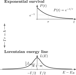
In the ideal exponential model, the $1/e$ probability lifetime is $\tau=\hbar/\Gamma$, while the Lorentzian energy profile has full width at half maximum $\Gamma$. The relation is exact only within the stated model and width convention.

The scattering-pole derivation, backgrounds, thresholds, and channel widths belong to Breit–Wigner Form. Spectral Functions owns the many-body conventions and the distinction among intrinsic, instrumental, and numerical broadening.

Why Exact Exponential Decay Cannot Be Universal

The ideal exponential is an effective law, usually accurate over an intermediate-time regime. Let

$$A(t) = \langle\psi| e^{-iHt/\hbar} |\psi\rangle$$

be the exact survival amplitude. If the required moments exist, its short-time expansion gives

$$|A(t)|^2 = 1 - \frac{(\Delta H)^2}{\hbar^2}t^2 + O(t^4).$$

The initial slope is zero. By contrast,

$$e^{-t/\tau} = 1-\frac{t}{\tau}+O(t^2)$$

has a nonzero initial slope. Exact unitary survival therefore begins quadratically when the energy variance is finite. This is the short-time regime underlying the quantum Zeno effect.

At very long times, a lower-bounded energy spectrum also obstructs a pure exponential extending forever. Threshold and spectral-edge structure generally produces nonexponential tails. Equivalently, an exact Lorentzian extending over the entire real energy axis is incompatible with a finite lower spectral bound.

Consequently, $\Gamma\tau=\hbar$ is a controlled relation for an isolated, approximately exponential resonance with a specified width convention. It is not a universal Robertson inequality for every decay process.

Finite-Time Windows and Fourier Resolution

A third source of energy–time language is ordinary Fourier analysis. Suppose an interaction is applied uniformly from $t=0$ to $t=T$. A first-order transition amplitude contains the window transform

$$\begin{aligned} F_T(\delta E) &= \int_0^T e^{i\delta E t/\hbar}\,dt \\ &= T e^{i\delta E T/(2\hbar)} \operatorname{sinc}\!\left( \frac{\delta E T}{2\hbar} \right), \end{aligned}$$

where

$$\operatorname{sinc}z = \frac{\sin z}{z}.$$

The squared amplitude has a central energy lobe of width proportional to $\hbar/T$. Its first zeros occur at

$$\delta E = \pm\frac{2\pi\hbar}{T}.$$

A short observation or pulse therefore has broad frequency content; a long window resolves a narrower energy difference. The exact numerical width depends on the window shape and on whether one quotes a standard deviation, half width, full width, or first-zero separation.

This is a bandwidth statement. At finite $T$, the sinc profile is not evidence that a closed system “borrows” energy. In a driven problem, the external control can exchange energy with the system. In the long-time limit, the increasingly narrow profile leads to the energy-selective delta distribution used in Fermi’s golden rule.

Measurement Duration Is a Separate Question

A proposed relation between an energy measurement error and the duration of the measurement requires a measurement model. At least four quantities must be kept separate:

• the preparation spread $\Delta_{\psi} H$ of the incoming state;
• the resolution or estimator error of the apparatus;
• the energy disturbance or transfer caused by the interaction;
• the clock time for which the interaction is active.

No universal Robertson theorem equates these quantities. Aharonov and Bohm gave measurement models showing that an arbitrarily short energy measurement need not obey a universal error-duration product of the naive form. Resource constraints, coupling strengths, control bandwidths, apparatus energy, and noise can produce useful model-dependent bounds, but those are additional physical assumptions.

Likewise, an arrival-time distribution or a quantum-clock reading can have its own uncertainty relation. Such a $\Delta t$ is defined by that clock or time POVM; it is not automatically the $\tau_A$, $T_\perp$, decay lifetime, or pulse duration defined elsewhere on this page.

Energy Conservation

For a closed system with a time-independent Hamiltonian,

$$\frac{d}{dt}\langle H\rangle = \frac{i}{\hbar}\langle[H,H]\rangle = 0.$$

The statement is stronger than conservation of the mean. If $P_H(B)$ is the spectral projector for an energy set $B$, then

$$\begin{aligned} p_H(B;t) &= \langle\psi(t)|P_H(B)|\psi(t)\rangle \\ &= \langle\psi(0)|P_H(B)|\psi(0)\rangle. \end{aligned}$$

The entire energy distribution is time independent because $P_H(B)$ commutes with the propagator generated by $H$.

For an explicitly time-dependent Hamiltonian,

$$\frac{d}{dt} \langle H(t)\rangle = \left\langle \frac{\partial H(t)}{\partial t} \right\rangle.$$

The changing external parameter performs work on the modeled system. A more complete description may include the drive or apparatus as additional quantum degrees of freedom, allowing conservation to be stated for the total closed system. Time-Dependent Hamiltonians develops this bookkeeping.

A subsystem can also exchange energy with its environment while the total energy is conserved. In perturbative language, an off-shell intermediate term is not a directly observed state temporarily exempt from conservation. The “borrowed energy” story confuses internal mathematical contributions, finite resolution, and physical asymptotic outcomes.

How to Read Any Energy–Time Formula

Before using a formula, identify each object explicitly.

What is the energy quantity?

It may be:

• a state standard deviation $\Delta H$;
• a mean excitation energy $\langle H\rangle-E_{\min}$;
• a resonance FWHM $\Gamma$;
• a detector resolution;
• a transition detuning $\delta E$;
• an energy transferred by a drive or environment.

What is the time quantity?

It may be:

• a local observable timescale $\tau_A$;
• a projective travel time or orthogonalization time $T_\perp$;
• a $1/e$ decay lifetime $\tau$;
• a pulse or observation duration $T$;
• an arrival-time or clock-reading uncertainty;
• a relaxation, decoherence, or correlation time.

Which hypotheses make the formula true?

Check whether the dynamics is closed or open, whether $H$ is time independent, whether the state is pure or mixed, whether the relevant moments are finite, which width convention is used, and which approximation produces the result. An unlabelled product $\Delta E\,\Delta t$ does not answer any of these questions.

Common Misstatements

“Energy conservation can be violated for a short time.”

No. For a closed system with time-independent $H$, the full energy distribution is constant. A drive or environment can exchange energy with a subsystem, and a finite time window has finite frequency resolution, but neither mechanism is a conservation-law loophole.

“Time is an observable exactly like position.”

Not in the standard formulation used here. Operational time observables exist, but there is no universal self-adjoint time operator canonically conjugate to every semibounded Hamiltonian.

“A process lasting $T$ has energy uncertainty exactly $\hbar/(2T)$.”

Not without definitions. A finite window produces a shape-dependent Fourier width; an evolving state may obey a speed limit; an apparatus may have a model-dependent resolution. Their constants and even their notions of width differ.

“Every state with a short lifetime has $\Delta H=\Gamma/2$.”

Not generally. An ideal Lorentzian has problematic high-energy tails and an undefined ordinary variance over the full real line. The resonance FWHM $\Gamma$ is not automatically the preparation standard deviation $\Delta H$.

“A stationary energy eigenvector does not evolve.”

Its vector acquires a phase, but its ray and all time-independent observable statistics are stationary. Physical state change is projective, not a change of an arbitrary vector phase.

Canonical Boundaries

• General Uncertainty Relations owns Robertson, Robertson–Schrödinger, equality conditions, and domain-safe formulations.
• Time as a Parameter owns the ordinary role of $t$, the spectral obstruction to a universal time operator, and specialized time observables.
• Fubini–Study Geometry owns the projective metric and the geometric derivation of state-space speed.
• Breit–Wigner Form owns the resonance pole, FWHM, backgrounds, thresholds, and channel widths.
• Spectral Functions owns many-body peak conventions and intrinsic versus extrinsic broadening.
• Stationary States owns the general energy-basis characterization of stationary evolution.

Summary

There is no context-free energy–time uncertainty formula. The most reusable core statements are:

$$\Delta H\,\tau_A \ge \frac\hbar2$$

for a defined observable-change timescale,

$$\int_0^T\Delta H(t)\,dt \ge \hbar \arccos \left\lvert \langle\psi(0)|\psi(T)\rangle \right\rvert$$

for pure-state projective evolution, and

$$\Gamma\tau = \hbar$$

for the explicitly defined exponential-decay and Lorentzian-FWHM model. Finite-time Fourier widths add another relation of order $\hbar/T$. These results are compatible because they refer to different energy quantities, different time quantities, and different hypotheses. None authorizes a temporary violation of energy conservation.

References

• L. Mandelstam and I. Tamm, “The uncertainty relation between energy and time in non-relativistic quantum mechanics,” Journal of Physics (USSR) 9, 249–254, 1945.
• Y. Aharonov and D. Bohm, “Time in the quantum theory and the uncertainty relation for time and energy,” Physical Review 122, 1649–1658, 1961, doi:10.1103/PhysRev.122.1649.
• G. N. Fleming, “A unitarity bound on the evolution of nonstationary states,” Il Nuovo Cimento A 16, 232–240, 1973, doi:10.1007/BF02819419.
• J. Anandan and Y. Aharonov, “Geometry of quantum evolution,” Physical Review Letters 65, 1697–1700, 1990, doi:10.1103/PhysRevLett.65.1697.
• N. Margolus and L. B. Levitin, “The maximum speed of dynamical evolution,” Physica D 120, 188–195, 1998, doi:10.1016/S0167-2789(98)00054-2.
• P. Busch, “The time–energy uncertainty relation,” in J. G. Muga, R. Sala Mayato, and I. L. Egusquiza, eds., Time in Quantum Mechanics, Springer, 2002, arXiv:quant-ph/0105049.
• L. A. Khalfin, “Contribution to the decay theory of a quasi-stationary state,” Soviet Physics JETP 6, 1053–1063, 1958.
• G. Breit and E. Wigner, “Capture of slow neutrons,” Physical Review 49, 519–531, 1936, doi:10.1103/PhysRev.49.519.
• S. Deffner and S. Campbell, “Quantum speed limits: from Heisenberg’s uncertainty principle to optimal quantum control,” Journal of Physics A 50, 453001, 2017, doi:10.1088/1751-8121/aa86c6.
• L. E. Ballentine, Quantum Mechanics: A Modern Development, 2nd ed., World Scientific, 2014.
• A. Peres, Quantum Theory: Concepts and Methods, Kluwer, 1995.
• J. J. Sakurai and J. Napolitano, Modern Quantum Mechanics, 3rd ed., Cambridge University Press, 2020.

Exercises

Exercise 1: Explicit time dependence

Starting from Robertson and the general expectation-value equation, prove

$$\Delta H\,\Delta A \ge \frac\hbar2 \left\lvert \frac{d}{dt}\langle A\rangle - \left\langle \frac{\partial A}{\partial t} \right\rangle \right\rvert.$$

Explain why replacing the right-hand side by $\frac\hbar2|d\langle A\rangle/dt|$ is not valid for every explicitly time-dependent observable.

Solution

Robertson applied to $H$ and $A$ gives

$$\Delta H\,\Delta A \ge \frac12 \left\lvert \langle[H,A]\rangle \right\rvert.$$

The expectation-value equation gives

$$\frac{i}{\hbar} \langle[H,A]\rangle = \frac{d}{dt}\langle A\rangle - \left\langle \frac{\partial A}{\partial t} \right\rangle.$$

Taking absolute values and substituting into Robertson proves the result. The total derivative contains both Hamiltonian-generated motion and explicit change in the operator. Robertson controls only the commutator contribution. An externally relabelled or moving observable can have a large total derivative even when $[H,A]=0$.

Exercise 2: Qubit observable timescale

For

$$H = \frac{\hbar\Omega}{2}\sigma_z, \qquad \lvert\psi(0)\rangle=\lvert+x\rangle,$$

compute $\langle\sigma_y\rangle_t$, $\Delta_t\sigma_y$, and $\tau_{\sigma_y}$. Verify saturation of the Mandelstam–Tamm observable bound whenever the timescale ratio is defined.

Solution

Rotation about the $z$ axis gives

$$\langle\sigma_y\rangle_t = \sin(\Omega t).$$

Since $\sigma_y^2=I$,

$$\Delta_t\sigma_y = \sqrt{1-\sin^2(\Omega t)} = |\cos(\Omega t)|.$$

The rate is

$$\left\lvert \frac{d}{dt}\langle\sigma_y\rangle_t \right\rvert = |\Omega|\,|\cos(\Omega t)|.$$

Thus $\tau_{\sigma_y}=1/|\Omega|$ when $\cos(\Omega t)\ne0$. Because the initial state gives equal probabilities for the two energy eigenvalues,

$$\Delta H = \frac{\hbar|\Omega|}{2}.$$

Therefore $\Delta H\,\tau_{\sigma_y}=\hbar/2$.

Exercise 3: Orthogonalization of two energy levels

Let

$$\lvert\psi(0)\rangle = \frac{\lvert E_0\rangle+\lvert E_1\rangle}{\sqrt2}, \qquad E_1>E_0.$$

Find the first time at which the state is orthogonal to its initial state and compare it with the Mandelstam–Tamm bound.

Solution

The overlap is

$$\begin{aligned} \langle\psi(0)|\psi(t)\rangle &= \frac12 e^{-iE_0t/\hbar} \\ &\quad+ \frac12 e^{-iE_1t/\hbar} \\ &= e^{-i(E_0+E_1)t/(2\hbar)} \\ &\quad\times \cos\!\left( \frac{(E_1-E_0)t}{2\hbar} \right). \end{aligned}$$

Its first zero occurs at

$$T_\perp = \frac{\pi\hbar}{E_1-E_0}.$$

The energy variance is that of two equally weighted outcomes:

$$\Delta H = \frac{E_1-E_0}{2}.$$

Hence

$$T_\perp = \frac{\pi\hbar}{2\Delta H},$$

so the bound is saturated.

Exercise 4: Degeneracy and stationarity

Suppose $\lvert a\rangle$ and $\lvert b\rangle$ are orthonormal eigenvectors with the same energy $E$. Show that every normalized superposition

$$\lvert\psi\rangle = \alpha\lvert a\rangle + \beta\lvert b\rangle$$

has zero energy spread and a stationary ray.

Solution

Linearity gives

$$H\lvert\psi\rangle = E\lvert\psi\rangle.$$

Therefore

$$\langle H\rangle=E, \qquad \langle H^2\rangle=E^2,$$

so $\Delta H=0$. Evolution is

$$\lvert\psi(t)\rangle = e^{-iEt/\hbar} \lvert\psi(0)\rangle.$$

All components acquire the same phase. The vector representative changes, but the ray and all time-independent observable probabilities remain fixed.

Exercise 5: Lifetime and FWHM

An isolated resonance has a $1/e$ probability lifetime $\tau=2.0\times10^{-9}\,\mathrm{s}$. In the ideal exponential model, compute its energy FWHM using

$$\hbar \simeq 6.582\times10^{-16}\,\mathrm{eV\,s}.$$

Solution

With the convention used on this page,

$$\Gamma = \frac\hbar\tau.$$

Therefore

$$\begin{aligned} \Gamma &= \frac{6.582\times10^{-16}\,\mathrm{eV\,s}} {2.0\times10^{-9}\,\mathrm{s}} \\ &\simeq 3.29\times10^{-7}\,\mathrm{eV}. \end{aligned}$$

This is the Lorentzian FWHM within the exponential model. It is not automatically the standard deviation of a normalized energy distribution.

Exercise 6: Short-time survival

For a normalized state with finite $\langle H^2\rangle$, expand

$$A(t) = \langle\psi|e^{-iHt/\hbar}|\psi\rangle$$

through second order and show that the survival probability has no term linear in $t$.

Solution

Expanding the exponential gives

$$A(t) = 1 - \frac{i\langle H\rangle}{\hbar}t - \frac{\langle H^2\rangle}{2\hbar^2}t^2 + O(t^3).$$

Multiplying by the complex conjugate yields

$$\begin{aligned} |A(t)|^2 &= 1 - \frac{ \langle H^2\rangle-\langle H\rangle^2 }{\hbar^2}t^2 + O(t^4) \\ &= 1 - \frac{(\Delta H)^2}{\hbar^2}t^2 + O(t^4), \end{aligned}$$

assuming enough moments for the displayed remainder. The linear terms cancel, so a pure exponential probability cannot be exact at arbitrarily short times.

Exercise 7: Rectangular time window

Evaluate

$$F_T(\delta E) = \int_0^T e^{i\delta E t/\hbar}\,dt$$

and find the nearest nonzero values of $\delta E$ for which it vanishes.

Solution

Direct integration gives

$$F_T(\delta E) = \frac{ e^{i\delta E T/\hbar}-1 }{i\delta E/\hbar}.$$

Factoring out the midpoint phase,

$$F_T(\delta E) = T e^{i\delta E T/(2\hbar)} \operatorname{sinc}\!\left( \frac{\delta E T}{2\hbar} \right).$$

The nearest nonzero roots of $\sin z$ are $z=\pm\pi$, so

$$\delta E = \pm\frac{2\pi\hbar}{T}.$$

This first-zero scale is proportional to $\hbar/T$. A different time window or width definition changes the numerical coefficient.

Exercise 8: Conservation diagnosis

For a closed state evolving under $H(t)$, derive

$$\frac{d}{dt}\langle H(t)\rangle = \left\langle \frac{\partial H(t)}{\partial t} \right\rangle.$$

Use it to distinguish a time-independent isolated system from a driven system.

Solution

Apply the general expectation-value equation with $A(t)=H(t)$:

$$\begin{aligned} \frac{d}{dt}\langle H(t)\rangle &= \frac{i}{\hbar} \\ &\quad\times \langle[H(t),H(t)]\rangle \\ &\quad+ \left\langle \frac{\partial H(t)}{\partial t} \right\rangle. \end{aligned}$$

The commutator vanishes, leaving the stated result. If $H$ has no explicit time dependence, the system’s mean energy is conserved. If $H(t)$ changes because an external control changes, the control can perform work on the system. A larger closed description can include that control and restore conservation for the total autonomous system. Neither case requires a temporary violation of an exact conservation law.